War of the Words | 🧬 Human vs 🅰👁️ Essay Detection

🥁 Introduction

This notebook explores the capability of machine learning algorithms to distinguish between essays written by humans and those generated by Large Language models.

⚠️ When programming automated judgment, which this indeed represents, it's beneficial to approach it with thoughtfulness and transparency. Understanding the reasons behind individual forecasts can add valuable insight alongside the specific methods used to generate these forecasts.

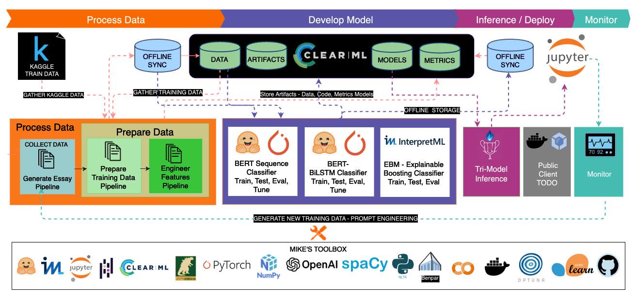
📐 Architecture

Using AWS ❝ Well-Architected Machine Learning Framework ❞ as a Guideline

Key Points:

• Design Philosophy: The architecture is aligned with the AWS 'Well-Architected Machine Learning' framework.
• Benefits:
  • Ready to scale up going forward
  • Ensures adherence to robust and efficient machine learning practices.

Importance:

• Best Practices: Aligns the project with industry standards in operational excellence, security, reliability, performance efficiency, and cost optimization.
• Future-Proofing: Even without current AWS implementation, this framework lays a strong foundation for potential AWS (and other cloud) integration.

Additional Resources:

• For a deeper understanding, visit AWS Well-Architected Machine Learning Framework.

🎮 Competition

https://www.kaggle.com/competitions/llm-detect-ai-generated-text

"Can you build a model to identify which essay was written by middle and high school students, and which was written using a large language model?"

"perhaps..."

📜 Hypothesis, Motivations and Objective

❈ Hypothesis: *Certain linguistic and structural patterns unique to AI-generated text can be identified and used for classification. We anticipate that our analysis will reveal distinct characteristics in AI-generated essays, enabling us to develop an effective classifier for this purpose.*

Motivations

• Learning and Challenge: Enhancing knowledge in Natural Language Processing (NLP) and staying intellectually active between jobs.
• Competition: https://www.kaggle.com/competitions/llm-detect-ai-generated-text
• Tool Development: Potential creation of a tool to differentiate between human and AI-generated content, useful across various fields.
• Educational Value: Serves as a practical introduction to production models in AI.

Objective

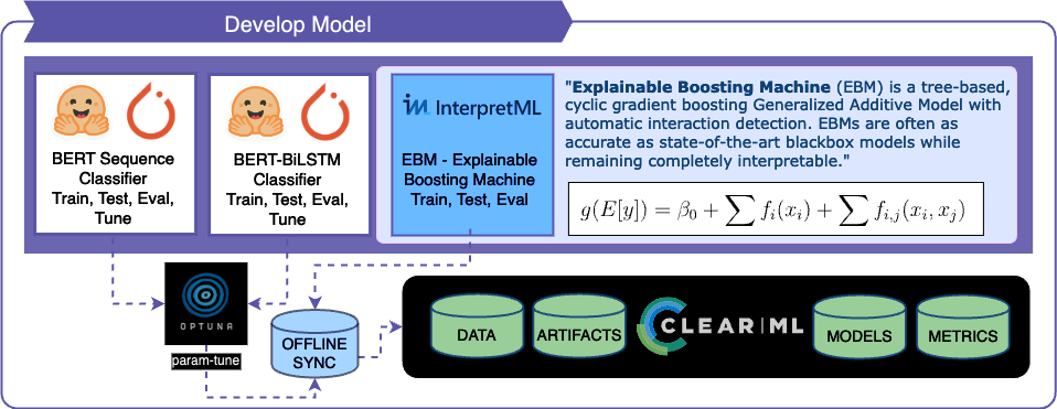
• Model Development: Building an ensemble model that combines two transformer models with an interpretable model like the Explainable Boosting Machine
• Challenges: Balancing effectiveness with interpretability.
• Approach:
  • Developing an Explainable Boosting Machine (EBM) that uses custom features to compliment BERT's performance with better interpretability.

♪📕s

Data:

• https://www.kaggle.com/datasets/geraltrivia/llm-detect-gpt354-generated-and-rewritten-essays
• https://www.kaggle.com/datasets/thedrcat/daigt-v2-train-dataset

Models:

• https://www.kaggle.com/code/geraltrivia/ai-human-pytorchbertsequenceclassifier-model
• https://www.kaggle.com/code/geraltrivia/ai-human-pytorchcustombertclassifier-model

note: these are the two models in this notebook. Had to train in another, it's too expensive to run all at once.

Notebooks: This code and the ClearML pipelines including the Essay Generation are here https://github.com/mikewlange/ai-or-human.

💡 ClearML Integration

"❤" - me

Strategic Choice and Benefits

• Purpose: ClearML integration to enhance workflow efficiency.
• Scalability and Efficiency: Focused on being prepared for scaling, even solo dev projects.
• Positive Experience: My experience with ClearML has been highly beneficial.

Implementation Details

• Pipelines Reference: In this project, all mentions of 'Pipelines' refer to ClearML pipelines.
• Resource Repository: A companion repository contains detailed code and examples for those interested in our ClearML implementation.

Impact of ClearML

• Operational Efficiency: ClearML has significantly improved the project's operational efficiency.
• Learning and Best Practices: It has also served as a platform for learning and applying best practices in ML operations, which is vital for scaling the project.

All the clearml related code is here: https://github.com/mikewlange/ai-or-human., but it's worth putting into the archtecture designs to help you see the whole picture.

✐ Setup for offline run

Kaggle Only

It's possible I'm doing this all wrong. To submit to a contest that disables the internet you neeed to add packages and other code/models that are not installed in the Kaggle docker image into a dataset (I.E storage) and use that as input to your notebook.

...

# turn off he internet and doing your pip installs, the packages you can't install, add to the libray var below 
      
      # TURN ON INTERNET FOR THIS
      # creates a wheelhouse to add 
      # 
      # library = \
      # '''
      # textstat
      # clearml
      # sentence_transformers 
      # optuna
      # interpret
      # torchsummary 
      # empath
      # benepar
      # '''.lstrip('\n')
      # with open('requirements.txt', 'w+') as f:
      #     f.write(library)
          
      #!mkdir wheelhouse && pip download -r requirements.txt -d wheelhouse
      
      # # Move requrements
      # !mv requirements.txt wheelhouse/requirements.txt
      
      ## Zip it up and then you can download
      # import os
      # from zipfile import ZipFile
      
      # dirName = "./"
      # zipName = "packages.zip"
      
      # # Create a ZipFile Object
      # with ZipFile(zipName, 'w') as zipObj:
      #     # Iterate over all the files in directory
      #     for folderName, subfolders, filenames in os.walk(dirName):
      #         for filename in filenames:
      #             if (filename != zipName):
      #                 # create complete filepath of file in directory
      #                 filePath = os.path.join(folderName, filename)
      #                 # Add file to zip
      #                 zipObj.write(filePath)
      # create a new dataset 
      # Take that zip file and add it to a dataset + button -> new dataset -> add all you need -> use as input here
      #TURN OFF INTERNET
      
      # wipe before any run. test. submission errors are no fun. 
      #!rm -rf /kaggle/working/*
      

⟴ Install Requirements

Kaggle Only

This is for files and libraries that are not in the kaggle docker runtime.

...

# !cp -r /kaggle/input/pip-installs/wheelhouse /kaggle/working/
      # !cp -r /kaggle/input/pip-installs/benepar_en3 /kaggle/working/
      
      # !pip install --no-index --find-links=/kaggle/working/wheelhouse /kaggle/working/wheelhouse/benepar-0.2.0/benepar-0.2.0
      
      # import sys 
      # sys.path.append("/kaggle/input/pip-installs/wheelhouse/sentence-transformers-2.2.2/sentence-transformers-2.2.2") 
      # import sentence_transformers 
      
      # sys.path.append("/kaggle/input/pip-installs/wheelhouse/empath-0.89/empath-0.89") 
      # from empath import Empath
      
      # # Creating this in realtime just in case we have to add-remove. 
      # requirements = """
      # textstat
      # clearml
      # optuna
      # interpret
      # torchsummary
      # """
      # with open('/kaggle/working/requirements.txt', 'w') as f:
      #     f.write(requirements)
          
      # ## install
      # !pip install -r /kaggle/working/requirements.txt --no-index --find-links /kaggle/input/pip-installs/wheelhouse
      # !pip install --no-index --find-links=/kaggle/working/wheelhouse torchsummary
      
      # # ## Prepare Benepar
      # import sys
      # import spacy
      # import benepar
      # import torchsummary
      # # fixes ealier issue
      # sys.path.insert(0, '/kaggle/working/')
      # nlp = spacy.load('en_core_web_lg') 
      # nlp.add_pipe("benepar", config={"model": "benepar_en3"})
      

✈️ Import Libraries

...

import pandas as pd
      import numpy as np
      import matplotlib.pyplot as plt
      import seaborn as sns
      import os
      import random
      import torch
      import logging
      from clearml.automation.controller import PipelineDecorator
      from clearml import TaskTypes, PipelineController, StorageManager, Dataset, Task
      from clearml import InputModel, OutputModel
      from IPython.display import display
      import ipywidgets as widgets
      from tqdm import tqdm
      import time
      import pickle
      
      import markdown
      from bs4 import BeautifulSoup
      import re
      import nltk
      from nltk.tokenize import word_tokenize
      from nltk.stem import WordNetLemmatizer
      

♽ Reproduceability

...

torch.manual_seed(42)
      if torch.cuda.is_available():
          torch.cuda.manual_seed(42)
          torch.backends.cudnn.deterministic = True
          torch.backends.cudnn.benchmark = False
      
      
      # Set random seed for NumPy
      np.random.seed(42)
      
      # Set random seed for random module
      random.seed(42)
      

⚙ Configuration

...

#os.environ['OPENAI_API_KEY'] = 
      
      class CFG:
          DEVICE = torch.device("cuda:0" if torch.cuda.is_available() else "cpu")
          CLEAR_ML_TRAINING_DATASET_ID = 'e71bc7e41b114a549ac1eaf1dff43099'  
          CLEAR_ML_KAGGLE_TRAIN_DATA = '24596ea241c34c6eb5013152a6122e48' 
          CLEAR_ML_AI_GENERATED_ESSAYS = '593fff56e3784e4fbfa4bf82096b0127'
          CLEAR_ML_AI_REWRITTEN_ESSAYS = '624315dd0e9b4314aa266654ebd71918'
          
          
          DATA_ETL_STRATEGY = 1
          TRAINING_DATA_COUNT = 50000
          CLEARML_OFFLINE_MODE = False
          CLEARML_ON = False
          KAGGLE_INPUT = '/kaggle/input'
          SCRATCH_PATH = 'scratch'
          ARTIFACTS_PATH = 'artifacts'
          TRANSFORMERS_PATH = 'benepar'
          ENSAMBLE_STRATEGY = 2
          KAGGLE_RUN = False
          SUBMISSION_RUN = True
          EXPLAIN_CODE=False
          BERT_MODEL = 'bert-base-uncased'
          EBM_ONLY = False
          RETRAIN=True
       
      
      cfg_dict = {key: value for key, value in CFG.__dict__.items() if not key.startswith('__')}
      
      feature_list = list()
      

⚒ Logging

A little logging class that integrates ClearML

...

import clearml
      class ClearMLTaskHandler:
          def __init__(self, project_name, task_name, config=None):
              self.task = self.get_or_create_task(project_name, task_name)
              self.logger = None  # Initialize logger attribute
              self.setup_widget_logger()
      
              if config:
                  self.set_config(config)
      
          def get_or_create_task(self, project_name, task_name):
              try:
                  tasks = []
                  if(CFG.CLEARML_OFFLINE_MODE):
                      Task.set_offline(offline_mode=True)
                  else:
                      tasks = Task.get_tasks(project_name=project_name, task_name=task_name)
                  
                  if tasks:
                      if(tasks[0].get_status() == "created" and task[0].task_name == task_name):
                          task = tasks[0]
                          return task
                      else:
                          if(CFG.CLEARML_OFFLINE_MODE):
                              Task.set_offline(offline_mode=True)
                              
                          task = Task.init(project_name=project_name, task_name=task_name)
                          return task
                  else:
                      if(CFG.CLEARML_OFFLINE_MODE):
                          Task.set_offline(offline_mode=True)
                          task = Task.init(project_name=project_name, task_name=task_name)
                      else:
                          task = Task.init(project_name=project_name, task_name=task_name)
                      return task
              except Exception as e:
                  print(f"Error occurred while searching for existing task: {e}")
                  return None
      
          def set_parameters(self, parameters):
              """
              Set hyperparameters for the task.
              :param parameters: Dictionary of parameters to set.
              """
              self.task.set_parameters(parameters)
      
          def set_config(self, config):
              if isinstance(config, dict):
                  self.task.connect(config)
              elif isinstance(config, argparse.Namespace):
                  self.task.connect(config.__dict__)
              elif isinstance(config, (InputModel, OutputModel, type, object)):
                  self.task.connect_configuration(config)
              else:
                  logging.warning("Unsupported configuration type")
      
          def log_data(self, data, title):
              self.task.get_logger()
              if isinstance(data, np.ndarray):
                  self.task.get_logger().report_image(title, 'array', iteration=0, image=data)
              elif isinstance(data, pd.DataFrame):
                  self.task.get_logger().report_table(title, 'dataframe', iteration=0, table_plot=data)
              elif isinstance(data, str) and os.path.exists(data):
                  self.task.get_logger().report_artifact(title, artifact_object=data)
              else:
                  self.task.get_logger().report_text(f"{title}: {data}")
          
          def upload_artifact(self, name, artifact):
              """
              Upload an artifact to the ClearML server.
              :param name: Name of the artifact.
              :param artifact: Artifact object or file path.
              """
              self.task.upload_artifact(name, artifact_object=artifact)
      
          def get_artifact(self, name):
              """
              Retrieve an artifact from the ClearML server.
              :param name: Name of the artifact to retrieve.
              :return: Artifact object.
              """
              return self.task.artifacts[name].get()
          
          def setup_widget_logger(self):
                  handler = OutputWidgetHandler()
                  handler.setFormatter(logging.Formatter('%(asctime)s  - [%(levelname)s] %(message)s'))
                  self.logger = logging.getLogger()  # Create a new logger instance
                  self.logger.addHandler(handler)
                  self.logger.setLevel(logging.INFO)
      
      
      # Just in case we can't use clearml in kaggle
      class OutputWidgetHandler(logging.Handler):
          def __init__(self, *args, **kwargs):
              super(OutputWidgetHandler, self).__init__(*args, **kwargs)
              layout = {'width': '100%', 'border': '1px solid black'}
              self.out = widgets.Output(layout=layout)
      
          def emit(self, record):
              formatted_record = self.format(record)
              new_output = {'name': 'stdout', 'output_type': 'stream', 'text': formatted_record+'\n'}
              self.out.outputs = (new_output, ) + self.out.outputs
      
          def show_logs(self):
              display(self.out)
      
          def clear_logs(self):
              self.out.clear_output()
      
      # Keeping this out for simpicity 
      def upload_dataset_from_dataframe(dataframe, new_dataset_name, dataset_project, description="", tags=[], file_name="dataset.pkl"):
          from pathlib import Path
          from clearml import Dataset
          import pandas as pd
          import logging
          try:
              print(dataframe.head())
              file_path = Path(file_name)
              pd.to_pickle(dataframe, file_path)
              new_dataset = Dataset.create(new_dataset_name,dataset_project, description=description)
              new_dataset.add_files(str(file_path))
              if description:
                  new_dataset.set_description(description)
              if tags:
                  new_dataset.add_tags(tags)
              new_dataset.upload()
              new_dataset.finalize()
              return new_dataset
          except Exception as e:
              return logging.error(f"Error occurred while uploading dataset: {e}")
          
      logging.basicConfig(level=logging.INFO)
      logger = logging.getLogger(__name__)
      

( ͡° ͜ʖ ͡°) 𝖘𝖍𝖆K𝖊𝖘𝖕𝖊𝖆𝖗𝖊 𝖜𝖗o𝖙𝖊 𝖈o𝖉𝖊

Ever find yourself snagging code snippets from Stack Overflow, ChatGPT, GitHub, or other treasure troves? You're not alone! But let's be honest, how many times have you wished the code was written in blank verse, composed in iambic pentameter with clever use of puns and imagery 🌹🌹 ? If so, it's your lucky day! [8]

⇟ Just toss explain_code(_i) into your cell, and voilà – it's like touching a hot stove. more info ⇟

[8] wikipedia

𝖘𝖍𝖆K𝖊𝖘𝖕𝖊𝖆𝖗𝖊?

• Deep Engagement: It encourages you to slow down and deeply engage with the content.
• Language Skill Enhancement: Instantly boosts your language skills. :)
• Programming and Language: Highlights the fact that programming is more about language than number crunching.
• Research Backing: Studies indicate that factors like fluid reasoning and language aptitude are crucial in understanding programming languages. [1]
• First Time: there is a good chance you've never read code explained like this.

𝖘𝖊T𝖚𝖕

1. Config Section Update:
   • Set your OpenAI API key: os.environ['OPENAI_API_KEY'] = 'your_key'.
   • In the CFG object, set EXPLAIN_CODE=True.
2. Code Explanation:
   • Add explain_code(_i) at the end of complex code cells.
3. Execution:
   • Run the cell and prepare for both enlightenment and a bit of humor.

from IPython.display import display, Markdown
      import ipywidgets as widgets 
      from openai import OpenAI
      client = OpenAI()
      model = "gpt-4-1106-preview"
      max_chars = 500
      
      def query_openai_api(model, cell_contents, max_chars=500):
          content = ""  # Initialize the content variable
      
          stream = client.chat.completions.create(
              model=model,
              response_format={"type": "text"},
              messages=[
                 {"role": "system", "content": cell_contents },
                  {"role": "user", "content": "Analyze the code in the system message. Give a 3 sentence brief. Use a mild shakespearean tone based on a random charater from one of shakespears plays . Then, display the rest of explanation as a Markdown bullet list. Do not use a greetings. Focus on brevity and clarity. "}
              ],
              max_tokens=max_chars,
              temperature=0.7,
              stream=True,
          )
          content = ""
          display(Markdown(content))
          for chunk in stream:
              content += chunk.choices[0].delta.content or ""
      
              if chunk.choices[0].finish_reason == "stop":
                  break
      
          display(Markdown(content))
      
      def explain_code(cell_contents):
          loading_icon = widgets.HTML(value="")  
          loading_icon.layout.display = "none"  # Hide the loading icon initially
          output = widgets.Output()
      
          def on_button_click(b):
              with output:
                  loading_icon.layout.display = "block"  # Show the loading icon
                  query_openai_api(model, cell_contents, max_chars)
                  loading_icon.layout.display = "none"  # Hide the loading icon
      
          button = widgets.Button(description="UNRAVEL MYSTERY",  tooltip="Click to explain the code in this cell using gpt-4-1106-preview")
          button.style.font_weight = "bold"
          hbox = widgets.HBox([button, loading_icon])
          button.background_color = "#05192D"
          button.button_style= "primary"
          button.style.width = "700px"
      
          button.on_click(on_button_click)
      
          display(hbox)
          display(output)
      
      if(CFG.EXPLAIN_CODE):
          explain_code(_i)
      

🤣 𝕰x𝖆M𝖕l𝖊 ↑ 🤣

❝ Verily, the script before us, a modern parchment, doth invoke the spirits of computation to unravel the mysteries enfolded within its characters. Like Prospero's conjuring of airs and whispers, this code beckons forth answers from the aether, seeking knowledge with a sprite's swiftness. Yet not with charms or spells, but with the silent tongues of Python and OpenAI's grand oracle, it reveals its secrets. ❞

• The script creates an interactive widget within a Jupyter notebook that allows users to submit Python code for analysis.
• Upon clicking the "UNRAVEL MYSTERY" button, the code is sent to the OpenAI API, which uses the GPT-4 model to generate an explanation of the provided code snippet.
• The explanation is then displayed within the notebook, styled in Markdown for ease of reading.
• The function query_openai_api is responsible for communicating with the OpenAI API, handling the response, and formatting it as Markdown content.
• A loading icon is displayed while the API processes the request, providing visual feedback that the operation is in progress.
• The explain_code function sets up the interactive components, including the button and output area, and handles the button click event.
• The on_button_click function is the event handler that triggers the API call and manages the display of the loading icon and output.

Note on Functionality

• Current Limitation: Presently, it works on a 'load-and-reveal' basis - I want it to stream.
• Future Updates: Would like to get the streaming to work. :)

✍ Generate Essays

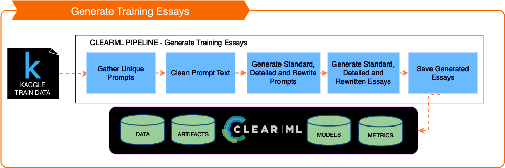
➠ Framework for Generating Essays

Quick overview. What are some ways students might use LLM's to conceal the origin of the essays?

1. Simple Topic Essay Nothing fancy, simple instructions and the prompt

Generate a quality and detailed middle or highschool essay that directly addresses the prompt: + prompt

2. Getting Creative Now we need to build a prompt that will fool the baseline model.

Generate an essay that closely resembles a high-quality, B+ level essay written by a 8th to 12th grade high-school student. The essay should reflect a deep understanding of the topic, with coherent arguments and clear structure. To closely mimic human writing, include subtle imperfections typical of a student at this level. These may include
- Occasional grammatical errors: Introduce minor grammatical mistakes that a student might make under exam conditions or in a final draft, such as slight misuse of commas, or occasional awkward phrasing.
- Varying sentence structure: Use a mix of simple, compound, and complex sentences, with some variation in fluency to reflect a student's developing writing style.
- Personal touch: Include personal opinions, anecdotes, or hypothetical examples where appropriate, to give the essay a unique voice.
- Argument depth: While the essay should be well-researched and informed, the depth of argument might not reach the sophistication of a more experienced writer. Arguments should be sound but might lack the nuance a more advanced writer would include.
- Conclusion: Ensure the essay has a clear conclusion, but one that might not fully encapsulate all the complexities of the topic, as a student might struggle to tie all threads together neatly.
Remember, the goal is to create a piece that balances high-quality content with the authentic imperfections of a human student writer. The essay should be on the following topic: + prompt

3. Rewrite Prompt That is where I would get caught. I love using AI to assist with rewrites and grammar checks.

Rewrite the following student essay by enhancing its structure, vocabulary, and overall quality. It's important to keep the same tone. Do not change facts or opinions. Ensure that the content and meaning of the original essay are preserved. Keep the lengths the same within 50 words: + prompt

Prompts were used from a competition dataset. https://www.kaggle.com/datasets/alejopaullier/daigt-external-dataset (original_moth)

The code for generating the essays is here: https://github.com/mikewlange/ai-or-human/blob/main/generate_essays_pipeline.ipynb

ClearML Task Setup

...

if(CFG.CLEARML_ON):
          clearml_handler = ClearMLTaskHandler(
              project_name='LLM-detect-ai-gen-text-LIVE/dev/notebook/preprocess',
              task_name='Load Data and Generate Features'
          )
      
          clearml_handler.set_parameters({'etl_strategy': cfg_dict['DATA_ETL_STRATEGY'], 'train_data_count': cfg_dict['TRAINING_DATA_COUNT']})
          clearml_handler.set_config(cfg_dict)
          task = clearml_handler.task
      

🚂 Prepare Training Data - Notebook Run

...

def download_dataset_as_dataframe(dataset_id='593fff56e3784e4fbfa4bf82096b0127', file_name="ai_generated.pkl"):
          import pandas as pd
          # import Dataset from clearml
          from clearml import Dataset
          dataset = Dataset.get(dataset_id, only_completed=True)
          cached_folder = dataset.get_local_copy()
          for file_name in os.listdir(cached_folder):
              if file_name.endswith('.pkl'):
                  file_path = os.path.join(cached_folder, file_name)
                  dataframe = pd.read_pickle(file_path)
                  return dataframe
          raise FileNotFoundError("No PKL file found in the dataset.")
      
      def download_dataset_as_dataframe_csv(dataset_id='593fff56e3784e4fbfa4bf82096b0127', file_name="ai_generated_essays.csv"):
          import pandas as pd
          # import Dataset from clearml
          extension = file_name.split('.')[-1]
          from clearml import Dataset
          dataset = Dataset.get(dataset_id, only_completed=True)
          cached_folder = dataset.get_local_copy()
          for file_name in os.listdir(cached_folder):
              if file_name.endswith(extension):
                  file_path = os.path.join(cached_folder, file_name)
                  dataframe = pd.read_csv(file_path)
                  return dataframe
              
      
              
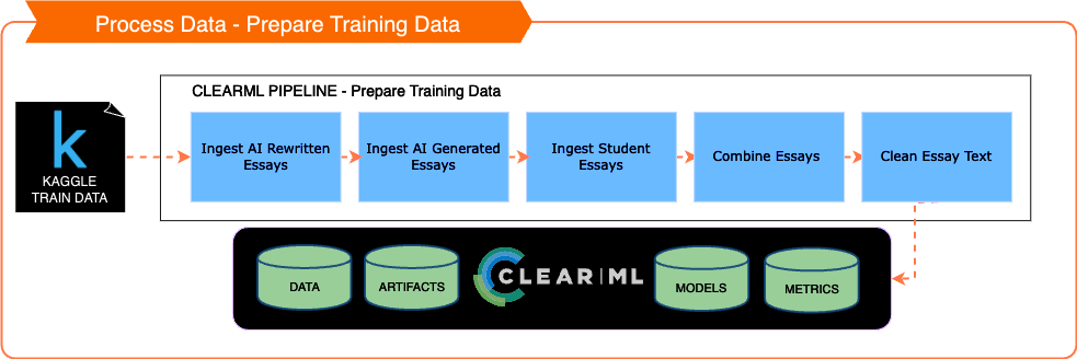
      kaggle_training_data = download_dataset_as_dataframe_csv(dataset_id=CFG.CLEAR_ML_KAGGLE_TRAIN_DATA,file_name="train_v2_drcat_02__final.csv")[['text','label','source']]
      ai_generated_essays = download_dataset_as_dataframe(dataset_id=CFG.CLEAR_ML_AI_GENERATED_ESSAYS,file_name="ai_generated.pkl")[['text','label','source']]
      ai_rewritten_essays = download_dataset_as_dataframe(dataset_id=CFG.CLEAR_ML_AI_REWRITTEN_ESSAYS,file_name="ai_rewritten_essays.pkl")[['text','label','source']]
      
      random_kaggle_training_data = kaggle_training_data[kaggle_training_data['label'] == 1].sample(n=10000) # from kaggle dataset
      random_generated_training_data = ai_generated_essays[ai_generated_essays['label'] == 1].sample(n=10000) # via the essay generation pipelint gpt3.5-4 essays written by AI and rewrittn
      kaggle_training_student = kaggle_training_data[kaggle_training_data['label'] == 0].sample(n=12000)
      
      random_kaggle_training_data = random_kaggle_training_data.dropna(subset=['text'])
      random_generated_training_data = random_generated_training_data.dropna(subset=['text'])
      kaggle_training_student = kaggle_training_student.dropna(subset=['text'])
      
      combined_data = pd.concat([random_generated_training_data,random_kaggle_training_data, kaggle_training_student], ignore_index=True)
      
      df_combined = combined_data.reset_index(drop=True)
      df_combined.drop_duplicates(inplace=True)
      
      df_essays = df_combined[['text', 'label', 'source']].copy()
      

Sample Training Data

...

sample = int(CFG.TRAINING_DATA_COUNT / 2)
      df_label_0 = df_essays[df_essays['label'] == 0].sample(n=2000, random_state=42)
      df_label_1 = df_essays[df_essays['label'] == 1].sample(n=2000, random_state=42) #<- example of data leakage 
      combined_df = pd.concat([df_label_1, df_label_0], ignore_index=True)
      combined_df = combined_df.dropna()
      df_essays = combined_df.reset_index(drop=True)
      

Plot Source and Label distribution

...

import plotly.graph_objects as go
      import matplotlib.pyplot as plt
      
      def plot_label_distribution(df_essays, plots, task=None):    
          if(plots == 1):
              label_1_counts = df_essays[df_essays['label'] == 1].groupby('source').size()
              label_0_counts = df_essays[df_essays['label'] == 0].groupby('source').size()
              data=[
                  go.Bar(name='Label 0', x=label_0_counts.index, y=label_0_counts.values),
                  go.Bar(name='Label 1', x=label_1_counts.index, y=label_1_counts.values)
              ]
              fig1 = go.Figure(data=data)
              fig1.update_layout(
                  title='Counts of Label 0 and Label 1 per Source',
                  xaxis_title='Source',
                  yaxis_title='Count',
                  barmode='group'
              )
              if(CFG.CLEARML_ON):          
                  task.get_logger().report_plotly(title="Counts of Label 0 and Label 1 per Source", series="data", figure=fig1)
                  
              # Show the chart using Plotly
              fig1.show()
              
          label_counts = df_essays['label'].value_counts().sort_index()
      
          print("Label Counts:")
          for label, count in label_counts.items():
              print(f"Label {label}: {count}")
      
          plt.bar(['0', '1'], label_counts.values)
          plt.xlabel('label')
          plt.ylabel('Count')
          plt.title('Distribution of label Values in df_essays')
          plt.show()
      
      plot_label_distribution(df_essays,1)
      
      if(CFG.EXPLAIN_CODE):
          explain_code(_i)
      

INFO:matplotlib.category:Using categorical units to plot a list of strings that are all parsable as floats or dates. If these strings should be plotted as numbers, cast to the appropriate data type before plotting.
      INFO:matplotlib.category:Using categorical units to plot a list of strings that are all parsable as floats or dates. If these strings should be plotted as numbers, cast to the appropriate data type before plotting.
      

Label Counts:
      Label 0: 2000
      Label 1: 2000
      

Clean Training Data

...

logging.basicConfig(level=logging.INFO, format='%(asctime)s - %(levelname)s - %(message)s')
      
      def pipeline_preprocess_text(df):
      
          PUNCTUATION_TO_RETAIN = '.?!,'
      
          def preprocess_pipeline(text):
              try:
                  # Remove markdown formatting
                  html = markdown.markdown(text)
                  text = BeautifulSoup(html, features="html.parser").get_text()
      
                  text = re.sub(r'[\n\r]+', ' ', text)
                  text = ' '.join(text.split())
      
                  text = re.sub(r'^(?:Task(?:\s*\d+)?\.?\s*)?', '', text)
                  text = re.sub('\n+', '', text)
                  text = re.sub(r'[A-Z]+_[A-Z]+', '', text)
       
                  punctuation_to_remove = r'[^\w\s' + re.escape(PUNCTUATION_TO_RETAIN) + ']'
                  text = re.sub(punctuation_to_remove, '', text)
      
                  tokens = word_tokenize(text)
                  lemmatizer = WordNetLemmatizer()
                  lemmatized_tokens = [lemmatizer.lemmatize(token) for token in tokens]
      
                  return ' '.join(lemmatized_tokens)
              except Exception as e:
                  logging.error(f"Error in preprocess_pipeline: {e}")
                  return text
      
          tqdm.pandas()
          start_time = time.time()
          df['text'] = df['text'].progress_apply(preprocess_pipeline)
          end_time = time.time()
          print(f"Preprocessing completed in {end_time - start_time:.2f} seconds")
      
          return df
      
      df_essays = pipeline_preprocess_text(df_essays)
      
      if(CFG.CLEARML_ON):
          plot_label_distribution(df_essays, 0, task=clearml_handler.task)
          clearml_handler.task.upload_artifact(f'df_essays_train_preprocessed_{CFG.DATA_ETL_STRATEGY}', artifact_object=df_essays)
          clearml_handler.task.get_logger().report_table(title='df_essays_train_preprocessed_',series='Train Essays Cleaned',
                                                      iteration=0,table_plot=df_essays)
      
      
      if(CFG.EXPLAIN_CODE):
          explain_code(_i)
      

  0%|          | 0/4000 [00:00<?, ?it/s]

100%|██████████| 4000/4000 [00:24<00:00, 160.03it/s]

Preprocessing completed in 25.01 seconds
      

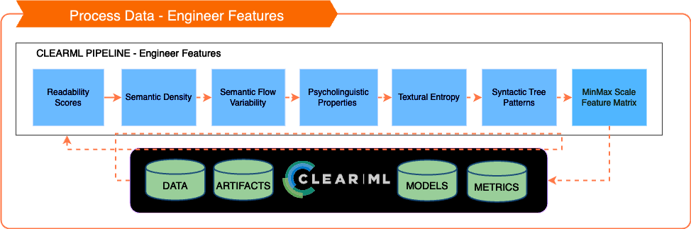
⁖ 📲 Engineer Features

For Feature Engineering, we focus on extracting attributes from the essay text data. In these features, we target capturing nuanced differences in textual characteristics, such as readability, semantic density, and syntactic patterns, distinguishing between AI-generated and human-written texts.

Key Analytical Areas

1. Readability Scores:

   • Identifying unique patterns in AI vs. human-written essays.
   • Analysis using scores like Flesch-Kincaid Grade Level, Gunning Fog Index, etc.

2. Semantic Density:

   • Understanding the concentration of meaning-bearing words in AI-generated vs. human text.

3. Semantic Flow Variability:

   • Examining idea transitions between sentences in human and AI-generated texts.

4. Psycholinguistic Features:

   • Using the LIWC tool for psychological and emotional content evaluation.

5. Textual Entropy:

   • Measuring unpredictability or randomness, focusing on differences between AI and human content.

6. Syntactic Tree Patterns:

   • Parsing essays to analyze syntactic tree patterns, especially structural tendencies in language models.

Ethical Considerations

• Content Bias: Ensuring to avoid generating discriminative content bias, focusing mainly on stat features.
• Potential Bias in Tools: Considering if tools like LIWC (empath) and the Readability Scores might introduce bias.

Note: These considerations are essential in maintaining the integrity and fairness of our analysis.

📊 Feature Distribution Statistics

Is there a statistacally signifigant difference in feature x's distribution betwen LLM and Human? Each of these measures provides a different perspective on the data, with the p-values offering insights into statistical significance and the effect size measures (Cohen's d and Glass's delta) providing information about the magnitude of the differences observed.

Example:

Understanding Key Statistical Concepts

1. T-Test p-value:

   • Purpose: Determines if differences between groups are statistically significant.
   • Interpretation: A low p-value (< 0.05) suggests significant differences, challenging the null hypothesis.

2. Mann-Whitney U p-value:

   • Usage: Ideal for non-normally distributed data, comparing two independent samples.
   • Significance: Similar to the T-test, a lower p-value indicates notable differences between the groups.

3. Kruskal-Wallis p-value:

   • Application: Used for comparing more than two independent samples.
   • Meaning: A low p-value implies significant variance in at least one of the samples from the others.

4. Cohen's d:

   • Function: Measures the standardized difference between two means.
   • Values: Interpreted as small (0.2), medium (0.5), or large (0.8) effects.

5. Glass's delta:

   • Comparison with Cohen's d: Similar in purpose but uses only the standard deviation of one group for normalization.
   • Utility: Effective when the groups' standard deviations differ significantly.

Note on Sample Size and Statistical Tests

• Small Samples (Under 5000 Records): T-Test, Mann-Whitney U, and Kruskal-Wallis tests are effective.
• Large Samples (Over 5000 Records): Focus on effect sizes (Cohen's d and Glass's delta), as p-values will generally approach 0.

...

def plot_feature_distribution(df_essays, categories_to_plot, show_plot=True):  
          import plotly.graph_objects as go
          import pandas as pd
          import numpy as np
          from scipy import stats
      
          def cohens_d(x, y):
              nx, ny = len(x), len(y)
              dof = nx + ny - 2
              return (np.mean(x) - np.mean(y)) / np.sqrt(((nx - 1) * np.std(x, ddof=1) ** 2 + (ny - 1) * np.std(y, ddof=1) ** 2) / dof)
      
          def glass_delta(x, y):
              return (np.mean(x) - np.mean(y)) / np.std(x, ddof=1)
      
          for category in categories_to_plot:
              df_filtered = df_essays[df_essays[category].astype(float) > 0]
              
              generated_0 = df_filtered[df_filtered["label"] == 0][category].astype(float)
              generated_1 = df_filtered[df_filtered["label"] == 1][category].astype(float)
      
              # Statistical tests and effect size calculations
              ttest_results = stats.ttest_ind(generated_0, generated_1, equal_var=False)
              d_value = cohens_d(generated_0, generated_1)
              delta_value = glass_delta(generated_0, generated_1)
              u_statistic, p_value = stats.mannwhitneyu(generated_0, generated_1, alternative="two-sided")
              k_statistic, p_value_k = stats.kruskal(generated_0, generated_1)
              
              # Log scalar metrics
              # logger.report_scalar(title="T-Test p-value", series=category, value=ttest_results.pvalue, iteration=0)
              # logger.report_scalar(title="Cohen's d", series=category, value=d_value, iteration=0)
              # logger.report_scalar(title="Glass's delta", series=category, value=delta_value, iteration=0)
              
              annotations = (
                  f"<b>T-Test p-value:</b> {ttest_results.pvalue:.2e} <b> Mann-Whitney U p-value:</b> {p_value:.2e}<br>"
                  f"<b>Kruskal-Wallis p-value:</b> {p_value_k:.2e} <b> Cohen's d:</b>{d_value:.2f} <b> Glass's delta:</b>{delta_value:.2f}<br><br><br>"
              )
      
              fig = go.Figure()
              data=[
                  go.Histogram(x=generated_0, name='Student', opacity=0.6),
                  go.Histogram(x=generated_1, name='AI', opacity=0.6)
              ]
              fig.add_trace(data[0])
              fig.add_trace(data[1])
      
              condition = False
              if (delta_value < -0.50) or (delta_value > 0.5):
                  condition = True
      
              txt = 'title'
              if condition:
                  title_text = f'<b>Distribution of {category.capitalize()}<span style="font-size: 30px; color: gold;">&#9733;</span></b>'
                  feature_list.append(category)
              else:
                  title_text = f'<b>Distribution of {category.capitalize()}</b>'
      
              fig.update_layout(
                  barmode='overlay',
                  title_text=title_text,
                  xaxis_title=f"{category.capitalize()}",
                  yaxis_title="Density",
                  annotations=[dict(
                      text=annotations,
                      x=.01,
                      y=-.25,
                      xref="paper",
                      yref="paper",
                      align="left",
                      showarrow=False,
                      bordercolor="#000000",
                      borderwidth=.3
                  )],
                  legend=dict(
                      orientation="v",
                      x=1.02,
                      y=1.0,
                      bgcolor="rgba(254, 255, 255, 0.5)",
                      bordercolor="#000000",
                      borderwidth=.3
                  ),
                  margin=dict(l=100, r=100, b=100)
              )
              if(show_plot):
                  fig.show()
      
              if(CFG.CLEARML_ON):          
                  Task.current_task().get_logger().report_plotly(title=f"{category.capitalize()}", series="data", figure=fig)
                  Task.current_task().get_logger().report_single_value("T-Test p-value: ",ttest_results.pvalue)
                  Task.current_task().get_logger().report_single_value("Mann-Whitney U p-value: ",p_value)
                  Task.current_task().get_logger().report_single_value("Cohen's d: ",d_value)
                  Task.current_task().get_logger().report_single_value("Glass's delta:",delta_value)
      

⁖ 📲 Features

ƒ(①) Readability Scores

We look at the Flesch-Kincaid Grade Level, Gunning Fog Index, Coleman-Liau Index,Automated Readability Index (ARI), Dale-Chall Readability Score scores of LLM-generated and human-written essays. The focus is on identifying distinct readability patterns characteristic of AI.

➠ Flesch-Kincaid Grade Level

This test gives a U.S. school grade level; for example, a score of 8 means that an eighth grader can understand the document. The lower the score, the easier it is to read the document. The formula for the Flesch-Kincaid Grade Level (FKGL) is:

$ FKGL = 0.39 \left( \frac{\text{total words}}{\text{total sentences}} \right) + 11.8 \left( \frac{\text{total syllables}}{\text{total words}} \right) - 15.59 $

Source: Wikipedia

➠ Gunning Fog Index

The Gunning Fog Index is a readability test designed to estimate the years of formal education a person needs to understand a text on the first reading. The index uses the average sentence length (i.e., the number of words divided by the number of sentences) and the percentage of complex words (words with three or more syllables) to calculate the score. The higher the score, the more difficult the text is to understand.

$ GunningFog = 0.4 \left( \frac{\text{words}}{\text{sentences}} + 100 \left( \frac{\text{complex words}}{\text{words}} \right) \right) $

In this formula:

• "Words" is the total number of words in the text.
• "Sentences" is the total number of sentences in the text.
• "Complex words" are words with three or more syllables, not including proper nouns, familiar jargon or compound words, or common suffixes such as -es, -ed, or -ing as a syllable.

The Gunning Fog Index is particularly useful for ensuring that texts such as technical reports, business communications, and journalistic works are clear and understandable for the intended audience.

Source: Wikipedia

➠ Coleman-Liau Index

The Coleman-Liau Index is a readability metric that estimates the U.S. grade level needed to comprehend a text. Unlike other readability formulas, it relies on characters instead of syllables per word, which can be advantageous for processing efficiency. The index is calculated using the average number of letters per 100 words and the average number of sentences per 100 words.

$ CLI = 0.0588 \times L - 0.296 \times S - 15.8 $

Where:

• L is the average number of letters per 100 words.
• S is the average number of sentences per 100 words.

Source: Wikipedia

➠ SMOG Index

The SMOG (Simple Measure of Gobbledygook) Index is a measure of readability that estimates the years of education needed to understand a piece of writing. It is calculated using the number of polysyllable words and the number of sentences. The SMOG Index is considered accurate for texts intended for consumers.

$ SMOG = 1.043 \times \sqrt{M \times \frac{30}{S}} + 3.1291 $

• M is the number of polysyllable words (words with three or more syllables).
• S is the number of sentences.

Source: Wikipedia

➠ Automated Readability Index (ARI)

The Automated Readability Index is a readability test designed to gauge the understandability of a text. The formula outputs a number that approximates the grade level needed to comprehend the text. The ARI uses character counts, which makes it suitable for texts with a standard character-per-word ratio.

$ ARI = 4.71 \times \left( \frac{\text{characters}}{\text{words}} \right) + 0.5 \times \left( \frac{\text{words}}{\text{sentences}} \right) - 21.43 $

Where:

• The number of characters is divided by the number of words.
• The number of words is divided by the number of sentences.

Source: wikipedia

➠ Dale-Chall Readability Score

The Dale-Chall Readability Score is unique in that it uses a list of words that are familiar to fourth-grade American students. The score indicates how many years of schooling someone would need to understand the text. If the text contains more than 5% difficult words (words not on the Dale-Chall familiar words list), a penalty is added to the score.

$ DaleChall = 0.1579 \times \left( \frac{\text{difficult words}}{\text{total words}} \times 100 \right) + 0.0496 \times \left( \frac{\text{total words}}{\text{sentences}} \right) $

$ \text{If difficult words} > 5\%: DaleChall = DaleChall + 3.6365 $

"Difficult words" are those not on the Dale-Chall list of familiar words.

Source: wikipedia

logging.basicConfig(level=logging.INFO)
      logger = logging.getLogger(__name__)
      tqdm.pandas()
      
      # Start time
      start_time = time.time()
      #@PipelineDecorator.component(return_values=["df"], name='Readability Scores', task_type=TaskTypes.data_processing)
      def process_readability_scores(df):
          import logging
          import textstat
          try:
              df['flesch_kincaid_grade'] = df['text'].progress_apply(textstat.flesch_kincaid_grade)
              df['gunning_fog'] = df['text'].progress_apply(textstat.gunning_fog)
              df['coleman_liau_index'] = df['text'].progress_apply(textstat.coleman_liau_index)
              df['smog_index'] = df['text'].progress_apply(textstat.smog_index)
              df['ari'] = df['text'].progress_apply(textstat.automated_readability_index)
              df['dale_chall'] = df['text'].progress_apply(textstat.dale_chall_readability_score)
              return df
          except Exception as e:
              logger.error(f"Error in process_readability_scores: {e}")
              raise
      %timeit
      df_essays = process_readability_scores(df_essays)
      
      end_time = time.time()
      
      duration = end_time - start_time
      
      print(f"Process completed in {duration:.2f} seconds")
      

  0%|          | 0/4000 [00:00<?, ?it/s]

100%|██████████| 4000/4000 [00:04<00:00, 996.32it/s] 
      100%|██████████| 4000/4000 [00:03<00:00, 1116.60it/s]
      100%|██████████| 4000/4000 [00:00<00:00, 4238.36it/s]
      100%|██████████| 4000/4000 [00:03<00:00, 1005.83it/s]
      100%|██████████| 4000/4000 [00:00<00:00, 4843.97it/s]
      100%|██████████| 4000/4000 [00:03<00:00, 1072.18it/s]

Process completed in 17.10 seconds
      

Plot Readability Score Statistics

categories_to_plot = [
                'flesch_kincaid_grade', 'gunning_fog', 'coleman_liau_index', 'smog_index', 'ari', 'dale_chall'
            ]
            condition = True  # Set the condition here
            
            plot_feature_distribution(df_essays, categories_to_plot,True)
            

ƒ(②) Semantic Density

Semantic Density refers to the concentration of meaning-bearing words within a text, a potential factor in differentiating between human-written and AI-generated essays. The process involves calculating the semantic density of essays by focusing on specific, meaning-rich parts of speech.

Calculating Semantic Density: The function calculate_semantic_density computes this metric by determining the ratio of meaning-bearing words (identified by tags in mb_tags) to the total word count. A higher semantic density indicates a text that efficiently uses words with substantial meaning.

import nltk
      from nltk.tokenize import word_tokenize
      import string
      # Start time
      start_time = time.time()
      
      def process_semantic_density(df):
          # Configure logging
          logging.basicConfig(level=logging.INFO, format='%(asctime)s - %(levelname)s - %(message)s')
      
      
          def get_meaning_bearing_tags():
              return {'NN', 'NNS', 'NNP', 'NNPS', 'VB', 'VBD', 'VBG', 'VBN', 'VBP', 'VBZ', 'JJ', 'JJR', 'JJS', 'RB', 'RBR', 'RBS'}
      
          def tokenize_text(text):
              try:
                  return word_tokenize(text.lower())
              except TypeError as e:
                  logging.error(f"Error tokenizing text: {e}")
                  return []
      
          def tag_words(words):
              try:
                  return nltk.pos_tag(words)
              except Exception as e:
                  logging.error(f"Error tagging words: {e}")
                  return []
      
          def filter_words(tokens):
              return [token for token in tokens if token.isalpha() or token in string.punctuation]
      
          mb_tags = get_meaning_bearing_tags()
      
          def process_row(text):
              tokens = tokenize_text(text)
              words = filter_words(tokens)
              tagged = tag_words(words)
              mb_words = [word for word, tag in tagged if tag in mb_tags]
              full_sentence = " ".join(word + "/" + tag for word, tag in tagged)
              density = len(mb_words) / len(words) if words else 0
              return density, full_sentence
      
          # Vectorized operations for DataFrame
          df[['semantic_density', 'text_tagged_nltk']] = df['text'].progress_apply(lambda x: pd.Series(process_row(x)))
      
          return df
      
      %timeit
      
      # run
      df_essays = process_semantic_density(df_essays)
      
      end_time = time.time()
      # Calculate duration
      duration = end_time - start_time
      print(f"Process completed in {duration:.2f} seconds")
      
      if(CFG.EXPLAIN_CODE):
          explain_code(_i)
      

  0%|          | 0/4000 [00:00<?, ?it/s]

100%|██████████| 4000/4000 [01:22<00:00, 48.31it/s]

Process completed in 82.80 seconds
      

Plot Semantic Density Statistics

categories_to_plot = [
                'semantic_density'
            ]
            condition = True  # Set the condition here
            plot_feature_distribution(df_essays, categories_to_plot,True)
            

ƒ(⓷) Semantic Flow Variability

This study examines the variation in semantic flow between sentences, a characteristic feature of human writing. For this analysis, the `all-MiniLM-L6-v2` model from Sentence Transformers is utilized. Renowned for its efficiency in transforming sentences and paragraphs into 384-dimensional vectors, this model is particularly adept for clustering and semantic search applications. Further details about the model can be found here.

The model's approach, based on contrastive learning, is key to its effectiveness. It excels in distinguishing sentence pairs from random samples, aligning closely with the study's objective to analyze semantic flow.

import concurrent.futures
      import logging
      import nltk
      import numpy as np
      from sentence_transformers import SentenceTransformer
      import torch
      from tqdm import tqdm
      tqdm.pandas()
      import time
      # Start time
      start_time = time.time()
      
      def process_semantic_flow_variability(df):
          logging.basicConfig(level=logging.INFO, format='%(asctime)s - %(levelname)s - %(message)s')
          logger = logging.getLogger(__name__)
          
      
          # Load a pre-trained sentence transformer model
          model_MiniLM = 'all-MiniLM-L6-v2' #https://huggingface.co/sentence-transformers/all-MiniLM-L6-v2
      
          try:
              model = SentenceTransformer(model_MiniLM)
          except Exception as e:
              logger.error(f"Error loading the sentence transformer model: {e}")
              model = None
      
          def cosine_similarity(v1, v2):
              return torch.dot(v1, v2) / (torch.norm(v1) * torch.norm(v2))
      
          def semantic_flow_variability(text):
              if not model:
                  logger.error("Model not loaded. Cannot compute semantic flow variability.")
                  return np.nan
      
              try:
                  sentences = nltk.sent_tokenize(text)
                  if len(sentences) < 2:
                      logger.info("Not enough sentences for variability calculation.")
                      return 0
      
                  sentence_embeddings = model.encode(sentences, convert_to_tensor=True, show_progress_bar=False)
      
                  # Calculate cosine similarity between consecutive sentences
                  similarities = [cosine_similarity(sentence_embeddings[i], sentence_embeddings[i+1])
                                  for i in range(len(sentence_embeddings)-1)]
      
      
                  return torch.std(torch.stack(similarities)).item()
      
      
              except Exception as e:
                  logger.error(f"Error calculating semantic flow variability: {e}")
                  return np.nan
      
          if df is not None and 'text' in df:
              # with concurrent.futures.ThreadPoolExecutor() as executor:
              df['semantic_flow_variability'] = df['text'].progress_apply(semantic_flow_variability)
          else:
              logger.error("Invalid DataFrame or missing 'text' column.")
      
          return df
      
      
      %timeit
      
      df_essays = process_semantic_flow_variability(df_essays)
      end_time = time.time()
      # Calculate duration
      duration = end_time - start_time
      print(f"Process completed in {duration:.2f} seconds")
      
      # Explain the code in the cell. Add this line to each cell
      if(CFG.EXPLAIN_CODE):
          explain_code(_i)
      

INFO:sentence_transformers.SentenceTransformer:Load pretrained SentenceTransformer: all-MiniLM-L6-v2
      INFO:sentence_transformers.SentenceTransformer:Use pytorch device: cpu
       20%|██        | 807/4000 [01:03<04:06, 12.94it/s]INFO:__main__:Not enough sentences for variability calculation.
       77%|███████▋  | 3099/4000 [04:01<01:01, 14.60it/s]INFO:__main__:Not enough sentences for variability calculation.
       87%|████████▋ | 3491/4000 [04:24<00:36, 13.97it/s]INFO:__main__:Not enough sentences for variability calculation.
      100%|██████████| 4000/4000 [04:55<00:00, 13.52it/s]
      

Process completed in 296.17 seconds
      

Plot Semantic Flow Variability Statistics

categories_to_plot = [
                'semantic_flow_variability'
            ]
            condition = True  # Set the condition here
            plot_feature_distribution(df_essays, categories_to_plot,True)
            

ƒ(⓸) Psycholinguistic Features

Psycholinguistic Features encompass the linguistic and psychological characteristics evident in speech and writing. These features provide insights into the writer's or speaker's psychological state, cognitive processes, and social dynamics. Analysis in this domain often involves scrutinizing word choice, sentence structure, and language patterns to deduce emotions, attitudes, and personality traits.

The Linguistic Inquiry and Word Count (LIWC) [3] is a renowned computerized text analysis tool that categorizes words into psychologically meaningful groups. It assesses various aspects of a text, including emotional tone, cognitive processes, and structural elements, covering categories like positive and negative emotions, cognitive mechanisms, and more.

While LIWC is typically accessible through purchase or licensing, this project will employ Empath, an open-source alternative to LIWC, to conduct similar analyses.

from empath import Empath
      import pandas as pd
      import logging
      
      # Initialize logging
      logging.basicConfig(level=logging.INFO)
      logger = logging.getLogger(__name__)
      
      # Create an Empath object
      lexicon = Empath()
      
      def empath_analysis(text):
          try:
              # Analyze the text with Empath and return normalized category scores
              analysis = lexicon.analyze(text, normalize=True)
              return analysis
          except Exception as e:
              # Log an error message if an exception occurs
              logger.error(f"Error during Empath analysis: {e}")
              # Return None or an empty dictionary to indicate failure
              return {}
      
      def apply_empath_analysis(df, text_column='text'):
          """
          Apply Empath analysis to a column in a DataFrame and expand the results into separate columns.
          """
          try:
              df['empath_analysis'] = df[text_column].apply(empath_analysis)
              empath_columns = df['empath_analysis'].apply(pd.Series)
              df = pd.concat([df, empath_columns], axis=1)
              df.drop(columns=['empath_analysis'], inplace=True)
              
              return df
          except Exception as e:
              # Log an error message if an exception occurs
              logger.error(f"Error applying Empath analysis to DataFrame: {e}")
              # Return the original DataFrame to avoid data loss
              return df
      
      df_essays = apply_empath_analysis(df_essays)
      
      # Explain the code in the cell. Add this line to each cell
      if(CFG.EXPLAIN_CODE):
          explain_code(_i)
      

Plot Psycholinguistic Feature Statistics

...

columns_to_scale = ['help','office','dance','money','wedding','domestic_work','sleep','medical_emergency','cold','hate','cheerfulness','aggression','occupation','envy','anticipation','family','vacation','crime','attractive','masculine','prison','health','pride','dispute','nervousness','government','weakness','horror','swearing_terms','leisure','suffering','royalty','wealthy','tourism','furniture','school','magic','beach','journalism','morning','banking','social_media','exercise','night','kill','blue_collar_job','art','ridicule','play','computer','college','optimism','stealing','real_estate','home','divine','sexual','fear','irritability','superhero','business','driving','pet','childish','cooking','exasperation','religion','hipster','internet','surprise','reading','worship','leader','independence','movement','body','noise','eating','medieval','zest','confusion','water','sports','death','healing','legend','heroic','celebration','restaurant','violence','programming','dominant_heirarchical','military','neglect','swimming','exotic','love','hiking','communication','hearing','order','sympathy','hygiene','weather','anonymity','trust','ancient','deception','fabric','air_travel','fight','dominant_personality','music','vehicle','politeness','toy','farming','meeting','war','speaking','listen','urban','shopping','disgust','fire','tool','phone','gain','sound','injury','sailing','rage','science','work','appearance','valuable','warmth','youth','sadness','fun','emotional','joy','affection','traveling','fashion','ugliness','lust','shame','torment','economics','anger','politics','ship','clothing','car','strength','technology','breaking','shape_and_size','power','white_collar_job','animal','party','terrorism','smell','disappointment','poor','plant','pain','beauty','timidity','philosophy','negotiate','negative_emotion','cleaning','messaging','competing','law','friends','payment','achievement','alcohol','liquid','feminine','weapon','children','monster','ocean','giving','contentment','writing','rural','positive_emotion','musical']
      
      plot_feature_distribution(df_essays, columns_to_scale,False) # too many, no need to view all. 
      

ƒ(⓹) Textual Entropy

Textual Entropy involves measuring the unpredictability or randomness in a text. It is a metric for distinguishing between AI-generated text and human writing, as each may exhibit distinct entropy characteristics.

The standard method for calculating entropy is outlined below, which evaluates the unpredictability of each character or word based on its frequency. This approach is encapsulated in the formula for Shannon Entropy:

$\begin{aligned} H(T) &= -\sum_{i=1}^{n} p(x_i) \log_2 p(x_i) &&\quad\text{(Shannon Entropy)} \\ \end{aligned}$

Shannon Entropy quantifies the level of information disorder or randomness, providing a mathematical framework to assess text complexity.

import numpy as np
      from collections import Counter
      import logging
      from tqdm import tqdm
      tqdm.pandas()
      import time
      # Start time
      start_time = time.time()
      # Configure logging
      logging.basicConfig(level=logging.INFO, format="%(asctime)s - %(levelname)s - %(message)s")
      logger = logging.getLogger(__name__)
      
      def calculate_entropy(text):
          """
          Calculate the Shannon entropy of a text string.
      
          Entropy is calculated by first determining the frequency distribution
          of the characters in the text, and then using these frequencies to
          calculate the probabilities of each character. The Shannon entropy
          is the negative sum of the product of probabilities and their log2 values.
      
          Args:
              text (str): The text string to calculate entropy for.
      
          Returns:
              float: The calculated entropy of the text, or 0 if text is empty/non-string.
              None: In case of an exception during calculation.
          """
          try:
              if not text or not isinstance(text, str):
                  logger.warning("Text is empty or not a string.")
                  return 0
      
              # Calculating frequency distribution and probabilities
              freq_dist = Counter(text)
              probs = [freq / len(text) for freq in freq_dist.values()]
              # Calculate entropy, avoiding log2(0)
              entropy = -sum(p * np.log2(p) for p in probs if p > 0)
              return entropy
          except Exception as e:
              logger.error(f"Error calculating entropy: {e}")
              return None
      
      %timeit
      try:
      
          df_essays["textual_entropy"] = df_essays["text"].progress_apply(calculate_entropy)
          end_time = time.time()
          duration = end_time - start_time
          print(f"Process completed in {duration:.2f} seconds")
      except Exception as e:
          logger.error(f"Error applying entropy calculation to DataFrame: {e}")
          end_time = time.time()
          duration = end_time - start_time
          print(f"Process completed in {duration:.2f} seconds")
      
      
      if(CFG.EXPLAIN_CODE):
          explain_code(_i)
      

100%|██████████| 4000/4000 [00:00<00:00, 6629.02it/s]

Process completed in 0.61 seconds
      

Plot Textual Entropy Stats

categories_to_plot = ['textual_entropy']
            plot_feature_distribution(df_essays, categories_to_plot,True)
            

ƒ(⓺) Syntactic Tree Patterns

Syntactic Tree Pattern Analysis The analysis involves parsing essays into syntactic trees to observe pattern frequencies and patterns, focusing on AI-generated and human-written text differences. This process employs the Berkeley Neural Parser, part of the Self-Attentive Parser[5][6] suite. The code is designed to parse natural language texts, specifically our essay data, using Natural Language Processing (NLP) techniques.

The function process_syntactic_tree_patterns is integral to this analysis. It utilizes spaCy, benepar, and NLTK to dissect the syntactic structures of texts, calculating metrics like tree depth, branching factors, nodes, leaves, and production rules. Additionally, it includes text analysis features like token length, sentence length, and entity analysis.

Features

1. num_sentences: Counts the total number of sentences in the text, providing an overview of text segmentation.

2. num_tokens: Tallies the total number of tokens (words and punctuation) in the text, reflecting the overall length.

3. num_unique_lemmas: Counts distinct base forms of words (lemmas), indicating the diversity of vocabulary used.

4. average_token_length: Calculates the average length of tokens, shedding light on word complexity and usage.

5. average_sentence_length: Determines the average number of tokens per sentence, indicating sentence complexity.

6. num_entities: Counts named entities (like people, places, organizations) recognized in the text, useful for understanding the focus and context.

7. num_noun_chunks: Tallies noun phrases, providing insights into the structure and complexity of nominal groups.

8. num_pos_tags: Counts the variety of parts of speech tags, reflecting grammatical diversity.

9. num_distinct_entities: Determines the number of unique named entities, indicative of the text's contextual richness.

10. average_entity_length: Calculates the average length of recognized entities, contributing to understanding the detail level of named references.

11. average_noun_chunk_length: Measures the average length of noun chunks, indicating the complexity and composition of noun phrases.

12. max_depth: Determines the maximum depth of syntactic trees in the text, a measure of syntactic complexity.

13. avg_branching_factor: Calculates the average branching factor of syntactic trees, reflecting the structural complexity and diversity.

14. total_nodes: Counts the total number of nodes in all syntactic trees, indicating the overall structural richness of the text.

15. total_leaves: Tallies the leaves in syntactic trees, correlated with sentence simplicity or complexity.

16. unique_rules: Counts the unique syntactic production rules found across all trees, indicative of syntactic variety.

17. tree_complexity: Measures the complexity of the syntactic trees by comparing the number of nodes to leaves.

18. depth_variability: Calculates the standard deviation of tree depths, indicating the variability in syntactic complexity across sentences.

These features collectively provide a comprehensive linguistic and structural analysis of the text, offering valuable insights into the syntactic and semantic characteristics of the processed essays.

...

import spacy
      import benepar
      import numpy as np
      import pandas as pd
      import logging
      from collections import Counter
      from nltk import Tree
      from transformers import T5TokenizerFast
      from tqdm import tqdm
      tqdm.pandas()
      import time
      # Start time
      #start_time = time.time()
      # Configure logging
      logging.basicConfig(level=logging.INFO, format='%(asctime)s - %(levelname)s - %(message)s')
      logger = logging.getLogger(__name__)
      import traceback
      
      def process_syntactic_tree_patterns(df_essays):
          start_time = time.time()
          """
          Process a DataFrame containing essays to extract various syntactic tree pattern features.
      
          The function uses spaCy, benepar, and NLTK to analyze syntactic structures of text,
          calculating various metrics such as tree depth, branching factors, nodes, leaves,
          and production rules. It also includes text analysis features like token length,
          sentence length, and entity analysis.
      
          Args:
              df_essays (pandas.DataFrame): DataFrame containing a 'text' column with essays.
      
          Returns:
              pandas.DataFrame: DataFrame with additional columns for each extracted syntactic and textual feature.
          """
          tokenizer = T5TokenizerFast.from_pretrained('t5-base', model_max_length=512, validate_args=False)
          
          
          try:
              nlp = spacy.load('en_core_web_lg') # Gotta use en_core_web_lg to use benepar_en3 for spacy 3.0
              # Just add the pipe. 
      #         nlp.add_pipe("benepar", config={"model": "benepar_en3"})
              if spacy.__version__.startswith('2'):
                  benepar.download('benepar_en3')
                  nlp.add_pipe(benepar.BeneparComponent("benepar_en3"))
              else:
                  nlp.add_pipe("benepar", config={"model": "benepar_en3"})
          except Exception as e:
              logger.error(f"Failed to load spaCy model: {e}")
              return df_essays
      
      
          def spacy_to_nltk_tree(node):
              if node.n_lefts + node.n_rights > 0:
                  return Tree(node.orth_, [spacy_to_nltk_tree(child) for child in node.children])
              else:
                  return node.orth_
      
          def tree_depth(node):
              if not isinstance(node, Tree):
                  return 0
              else:
                  return 1 + max(tree_depth(child) for child in node)
      
          def tree_branching_factor(node):
              if not isinstance(node, Tree):
                  return 0
              else:
                  return len(node)
      
          def count_nodes(node):
              if not isinstance(node, Tree):
                  return 1
              else:
                  return 1 + sum(count_nodes(child) for child in node)
      
          def count_leaves(node):
              if not isinstance(node, Tree):
                  return 1
              else:
                  return sum(count_leaves(child) for child in node)
      
          def production_rules(node):
              rules = []
              if isinstance(node, Tree):
                  rules.append(node.label())
                  for child in node:
                      rules.extend(production_rules(child))
              return rules
      
          def count_labels_in_tree(tree, label):
              if not isinstance(tree, Tree):
                  return 0
              count = 1 if tree.label() == label else 0
              for subtree in tree:
                  count += count_labels_in_tree(subtree, label)
              return count
      
          def count_phrases_by_label(trees, label, doc):
              if label == 'NP':
                  noun_phrases = [chunk.text for chunk in doc.noun_chunks]
                  return noun_phrases
              else:
                  return sum(count_labels_in_tree(tree, label) for tree in trees if isinstance(tree, Tree))
      
          def count_subtrees_by_label(trees, label):
              return sum(count_labels_in_tree(tree, label) for tree in trees if isinstance(tree, Tree))
      
          def average_phrase_length(trees):
              lengths = [len(tree.leaves()) for tree in trees if isinstance(tree, Tree)]
              return np.mean(lengths) if lengths else 0
      
          def subtree_height(tree, side):
              if not isinstance(tree, Tree) or not tree:
                  return 0
              if side == 'left':
                  return 1 + subtree_height(tree[0], side)
              elif side == 'right':
                  return 1 + subtree_height(tree[-1], side)
      
          def average_subtree_height(trees):
              heights = [tree_depth(tree) for tree in trees if isinstance(tree, Tree)]
              return np.mean(heights) if heights else 0
      
          def pos_tag_distribution(trees):
              pos_tags = [tag for tree in trees for word, tag in tree.pos()]
              return Counter(pos_tags)
      
          def process_tree_or_string(obj):
              if isinstance(obj, Tree):
                  return obj.height()
              else:
                  return None
      
          def syntactic_ngrams(tree):
              ngrams = []
              if isinstance(tree, Tree):
                  ngrams.extend(list(nltk.ngrams(tree.pos(), 2)))
              return ngrams
          
      
          for index, row in df_essays.iterrows():
              text = row['text']
              try:
                  doc = nlp(text)
                  trees = [spacy_to_nltk_tree(sent.root) for sent in doc.sents if len(tokenizer.tokenize(sent.text)) < 512]
                  trees = [tree for tree in trees if isinstance(tree, Tree)]
      
                  # Extract features
                  depths = [tree_depth(tree) for tree in trees if isinstance(tree, Tree)]
                  branching_factors = [tree_branching_factor(tree) for tree in trees if isinstance(tree, Tree)]
                  nodes = [count_nodes(tree) for tree in trees if isinstance(tree, Tree)]
                  leaves = [count_leaves(tree) for tree in trees if isinstance(tree, Tree)]
                  rules = [production_rules(tree) for tree in trees if isinstance(tree, Tree)]
                  rule_counts = Counter([rule for sublist in rules for rule in sublist])
      
                  # Text analysis features
                  num_sentences = len(list(doc.sents))
                  num_tokens = len(doc)
                  unique_lemmas = set([token.lemma_ for token in doc])
                  total_token_length = sum(len(token.text) for token in doc)
                  average_token_length = total_token_length / num_tokens if num_tokens > 0 else 0
                  average_sentence_length = num_tokens / num_sentences if num_sentences > 0 else 0
                  num_entities = len(doc.ents)
                  num_noun_chunks = len(list(doc.noun_chunks))
                  pos_tags = [token.pos_ for token in doc]
                  num_pos_tags = len(set(pos_tags))
                  distinct_entities = set([ent.text for ent in doc.ents])
                  total_entity_length = sum(len(ent.text) for ent in doc.ents)
                  average_entity_length = total_entity_length / num_entities if num_entities > 0 else 0
                  total_noun_chunk_length = sum(len(chunk.text) for chunk in doc.noun_chunks)
                  average_noun_chunk_length = total_noun_chunk_length / num_noun_chunks if num_noun_chunks > 0 else 0
                  ngrams = []
                  for tree in trees:
                      ngrams.extend(syntactic_ngrams(tree))
      
                  # Assign calculated feature values to the DataFrame
                  df_essays.at[index, 'num_sentences'] = num_sentences
                  df_essays.at[index, 'num_tokens'] = num_tokens
                  df_essays.at[index, 'num_unique_lemmas'] = len(unique_lemmas)
                  df_essays.at[index, 'average_token_length'] = average_token_length
                  df_essays.at[index, 'average_sentence_length'] = average_sentence_length
                  df_essays.at[index, 'num_entities'] = num_entities
                  df_essays.at[index, 'num_noun_chunks'] = num_noun_chunks
                  df_essays.at[index, 'num_pos_tags'] = num_pos_tags
                  df_essays.at[index, 'num_distinct_entities'] = len(distinct_entities)
                  df_essays.at[index, 'average_entity_length'] = average_entity_length
                  df_essays.at[index, 'average_noun_chunk_length'] = average_noun_chunk_length
                  df_essays.at[index, 'max_depth'] = max(depths) if depths else 0
                  df_essays.at[index, 'avg_branching_factor'] = np.mean(branching_factors) if branching_factors else 0
                  df_essays.at[index, 'total_nodes'] = sum(nodes)
                  df_essays.at[index, 'total_leaves'] = sum(leaves)
                  df_essays.at[index, 'unique_rules'] = len(rule_counts)
                  df_essays.at[index, 'most_common_rule'] = rule_counts.most_common(1)[0][0] if rule_counts else None
                  df_essays.at[index, 'tree_complexity'] = sum(nodes) / sum(leaves) if leaves else 0
                  df_essays.at[index, 'depth_variability'] = np.std(depths)
                  #df_essays.at[index, 'subtree_freq_dist'] = Counter([' '.join(node.leaves()) for tree in trees for node in tree.subtrees() if isinstance(node, Tree)])
                  df_essays.at[index, 'tree_height_variability'] = np.std([subtree_height(tree, 'left') for tree in trees if isinstance(tree, Tree)])
                  
                  #df_essays.at[index, 'pos_tag_dist'] = pos_tag_distribution(trees)
                  #df_essays.at[index, 'syntactic_ngrams'] = ngrams
      
              except Exception as e:
                  logger.error(f"Error processing text: {e}")
                  traceback.print_exc()
                  # Assign NaNs in case of error
                  # df_essays.at[index, 'num_sentences'] = np.nan
                  # ... Assign NaNs for other features ...
      
          return df_essays
      
      #%timeit
      # Usage
      try:
          print("Step 7: process_syntactic_tree_patterns")
          df_essays = process_syntactic_tree_patterns(df_essays)
          
          end_time = time.time()
          # Calculate duration
          duration = end_time - start_time
      except Exception as e:
          logger.error(f"ERROR: process_syntactic_tree_patterns: {e}")
      
      # Explain the code in the cell. Add this line to each cell
      if(CFG.EXPLAIN_CODE):
          explain_code(_i)
      

Step 7: process_syntactic_tree_patterns
      

You're using a T5TokenizerFast tokenizer. Please note that with a fast tokenizer, using the `__call__` method is faster than using a method to encode the text followed by a call to the `pad` method to get a padded encoding.
      /Users/lange/anaconda3/envs/py39/lib/python3.9/site-packages/torch/distributions/distribution.py:53: UserWarning:
      
      <class 'torch_struct.distributions.TreeCRF'> does not define `arg_constraints`. Please set `arg_constraints = {}` or initialize the distribution with `validate_args=False` to turn off validation.
      
      /Users/lange/anaconda3/envs/py39/lib/python3.9/site-packages/torch/distributions/distribution.py:53: UserWarning:
      
      <class 'torch_struct.distributions.TreeCRF'> does not define `arg_constraints`. Please set `arg_constraints = {}` or initialize the distribution with `validate_args=False` to turn off validation.
      
      

Plot Syntactic Tree Pattern Statistics

categories_to_plot = ['num_sentences','num_tokens','num_unique_lemmas','average_token_length','average_sentence_length','num_entities','num_noun_chunks','num_pos_tags','num_distinct_entities','average_entity_length','average_noun_chunk_length','max_depth','avg_branching_factor','total_nodes','total_leaves','unique_rules','tree_complexity','depth_variability']
            plot_feature_distribution(df_essays, categories_to_plot,True)
            

⓻ Scale features for EBM training

we use a MinMaxScaler and scale each 'group' individually.

...

def sanity_check():
          columns_with_nan = df_essays.columns[df_essays.isna().any()].tolist()
          nan_count = df_essays[columns_with_nan].isna().sum()
          print(nan_count)
          for column, count in zip(columns_with_nan, nan_count):
              print(f"Column '{column}' has {count} NaN value(s).")
          assert nan_count.sum() == 0, "NaN values found in the DataFrame."
          print("There are no missing values in df_essays.")
      df_essays.dropna(inplace=True)
      sanity_check() 
      

Series([], dtype: float64)
      There are no missing values in df_essays.
      

# Create a deep copy so i can use the original df_essays later
      df_essays_copy = df_essays.copy(deep=True) ## for now
      

from sklearn.preprocessing import MinMaxScaler, StandardScaler
      
      
      def scale_columns(df, columns_to_scale, scaler=None, scale_type='MinMaxScaler'):
          """
          Scale the specified columns in a DataFrame and add a suffix to the column names.
      
          Args:
              df (pandas.DataFrame): The DataFrame to scale.
              columns_to_scale (list): List of column names to scale.
              scaler (object, optional): Scaler object to use for scaling. If None, a new scaler object will be created.
              scale_type (str, optional): The type of scaler to use. Default is 'MinMaxScaler'. Options: 'MinMaxScaler', 'StandardScaler'.
      
          Returns:
              pandas.DataFrame: The full DataFrame with scaled columns added.
              pandas.DataFrame: A separate DataFrame with only the specified columns scaled.
              object: The scaler object used for scaling.
          """
          if scale_type == 'MinMaxScaler':
              scaler = MinMaxScaler() if scaler is None else scaler
          elif scale_type == 'StandardScaler':
              scaler = StandardScaler() if scaler is None else scaler
          else:
              raise ValueError("Invalid scale_type. Options: 'MinMaxScaler', 'StandardScaler'")
      
          scaled_columns = scaler.fit_transform(df[columns_to_scale])
          scaled_df = pd.DataFrame(scaled_columns, columns=[col + '_scaled' for col in columns_to_scale])
      
          full_df = pd.concat([df.drop(columns=columns_to_scale), scaled_df], axis=1)
      
          return full_df, scaled_df, scaler
      

Scale Readability Scores

import joblib
      columns_to_scale = ['flesch_kincaid_grade', 'gunning_fog', 'coleman_liau_index', 'smog_index', 'ari', 'dale_chall', 'textual_entropy', 'semantic_density', 'semantic_flow_variability']
      readability_scaled_backin_df, readability_scaled_df, readability_scaler = scale_columns(df_essays_copy, columns_to_scale, scale_type='MinMaxScaler')
      joblib.dump(readability_scaler, f'{CFG.SCRATCH_PATH}/scaler_semantic_features.pkl', compress=True)
      

['scratch/scaler_semantic_features.pkl']

Scale Psycholinguistic Features

columns_to_scale = ['help','office','dance','money','wedding','domestic_work','sleep','medical_emergency','cold','hate','cheerfulness','aggression','occupation','envy','anticipation','family','vacation','crime','attractive','masculine','prison','health','pride','dispute','nervousness','government','weakness','horror','swearing_terms','leisure','suffering','royalty','wealthy','tourism','furniture','school','magic','beach','journalism','morning','banking','social_media','exercise','night','kill','blue_collar_job','art','ridicule','play','computer','college','optimism','stealing','real_estate','home','divine','sexual','fear','irritability','superhero','business','driving','pet','childish','cooking','exasperation','religion','hipster','internet','surprise','reading','worship','leader','independence','movement','body','noise','eating','medieval','zest','confusion','water','sports','death','healing','legend','heroic','celebration','restaurant','violence','programming','dominant_heirarchical','military','neglect','swimming','exotic','love','hiking','communication','hearing','order','sympathy','hygiene','weather','anonymity','trust','ancient','deception','fabric','air_travel','fight','dominant_personality','music','vehicle','politeness','toy','farming','meeting','war','speaking','listen','urban','shopping','disgust','fire','tool','phone','gain','sound','injury','sailing','rage','science','work','appearance','valuable','warmth','youth','sadness','fun','emotional','joy','affection','traveling','fashion','ugliness','lust','shame','torment','economics','anger','politics','ship','clothing','car','strength','technology','breaking','shape_and_size','power','white_collar_job','animal','party','terrorism','smell','disappointment','poor','plant','pain','beauty','timidity','philosophy','negotiate','negative_emotion','cleaning','messaging','competing','law','friends','payment','achievement','alcohol','liquid','feminine','weapon','children','monster','ocean','giving','contentment','writing','rural','positive_emotion','musical']
      psycho_scaled_df_backin_df, psycho_scaled_df, psycho_scaler = scale_columns(df_essays_copy, columns_to_scale, scale_type='MinMaxScaler')
      joblib.dump(psycho_scaler, f'{CFG.SCRATCH_PATH}/scaler_psycho_features.pkl', compress=True)
      

['scratch/scaler_psycho_features.pkl']

Scale Tree Features

columns_to_scale = ['num_sentences', 'num_tokens', 'num_unique_lemmas', 'average_token_length', 'average_sentence_length', 'num_entities', 'num_noun_chunks', 'num_pos_tags', 'num_distinct_entities', 'average_entity_length', 'average_noun_chunk_length', 'max_depth', 'avg_branching_factor', 'total_nodes', 'total_leaves', 'unique_rules', 'tree_complexity', 'depth_variability']
      tree_feature_scaler_backin_df, tree_features_scaled_df, tree_feature_scaler = scale_columns(df_essays_copy, columns_to_scale, scale_type='MinMaxScaler')
      joblib.dump(tree_feature_scaler, f'{CFG.SCRATCH_PATH}/scaler_tree_features.pkl', compress=True)
      

['scratch/scaler_tree_features.pkl']

Combine Scaled Features

final_features_df = pd.concat([readability_scaled_df,tree_features_scaled_df,psycho_scaled_df], axis=1)
      print("Shape df_essays_copy: " + str(df_essays_copy.shape))
      print("Semantic Features Scaled: " + str(final_features_df.shape))
      
      #final_features_df.head()
      

Shape df_essays_copy: (3999, 227)
      Semantic Features Scaled: (3999, 221)
      

ClearML Features Close

if(CFG.CLEARML_ON):
          # These are the final before uploading and starting the modeling process. 
          upload_dataset_from_dataframe(final_features_df,"training_with_features_scaled",
                                                        'LLM-detect-ai-gen-text-LIVE/dev/notebook/preprocess',
                                                        "Training Data with Features, Post the scaling",
                                                        ["training_with_features_scaled","feature"],
                                                        "scratch/training_with_features_scaled.pkl")
      
          upload_dataset_from_dataframe(df_essays_copy,"training_with_features",
                                                    'LLM-detect-ai-gen-text-LIVE/dev/notebook/preprocess',
                                                    "Training Data with Features, Before Scaling",
                                                    ["training_with_features","feature"],
                                                    "scratch/training_with_features.pkl")
        
          clearml_handler.task.get_logger().report_table(title='training_with_features_scaled',series='Train Essays Features',
                                                      iteration=0,table_plot=final_features_df)
          clearml_handler.task.close()
      

🧮 Model Development

Model Overview

1. BertForSequenceClassification:

   • Architecture: BERT (Bidirectional Encoder Representations from Transformers) for sequence classification. [4]
   • Process: Involves data pre-processing, data loading, and training with hyperparameter optimization.
   • Metrics: Trained and monitored using accuracy, precision, recall, F1 score, and AUC.

2. BertModel + BiLSTM:

   • Architecture: The model is composed of the BertModel layer followed by BiLSTM layers. This is further connected to a dropout layer for regularization, a fully connected linear layer with ReLU activation, and a final linear layer for classification.

3. Explainable Boosting Machine (EBM) for Feature Classification:

   • Type: Glass-box model, notable for interpretability and effectiveness.
   • Function: Classifies based on extracted features from the essays.
   • Configuration: Includes settings for interaction depth, learning rate, and validation size.
   • Insights: Provides understanding of feature importance and model behavior.
   • Causality This is a 'casual' model and the EBM is for helping dertermine causality aloong with our feature stats

Ensemble Approach

• Final Output Calculation: The outputs of each model are summed and then averaged to determine the ensemble's final output.

Sanity Check

...

def sanity_check_2():
          # Check the number of missing values
          assert final_features_df.isnull().sum().sum() == 0, "There are missing values in final_features_df."
          print("There are no missing values in final_features_df.")
      
          # Check the data types
          assert final_features_df.dtypes.unique().tolist() == [np.float64], "The data types of final_features_df are incorrect."
          print("Data types of final_features_df are correct.")
      
          # compare row count and assert on error 
          assert df_essays_copy.shape[0] == final_features_df.shape[0], "Row count mismatch between df_essays_copy and final_features_df"
          print("Row count between df_essays_copy and final_features_df is correct")
          # Check the range of values
          # assert final_features_df.max().max() <= 1 and final_features_df.min().min() >= 0, "The values in final_features_df are not between 0 and 1."
          # print("All values in final_features_df are between 0 and 1.")
      
      sanity_check_2()  # I had to take a week off after sanity_check_1() :)
      

There are no missing values in final_features_df.
      Data types of final_features_df are correct.
      Row count between df_essays_copy and final_features_df is correct
      

🤗 BERT for Sequence Classification

bert-base-uncased

Leveraging the 🤗 bert-base-uncased model, this section integrates the BertForSequenceClassification for efficient text sequence classification, combining BERT's advanced language processing with a streamlined, single-layer architecture for optimal simplicity and efficacy

Overview

• Model Type: BertForSequenceClassification, adapted from the pre-trained BERT model.
• Architecture: Integrates BERT's transformer layers with a single linear layer for classification.
• Design Advantage: Leverages BERT's advanced language understanding while ensuring efficiency in classification tasks.

Rationale

• Pre-trained Foundation: Utilizes the foundational BERT model pre-trained on a vast corpus. This approach leverages existing rich text representations, reducing the need for extensive training data and time.
• Simplicity and Efficiency Balance: Achieves a balance between simplicity and operational efficiency. The single linear layer addition to BERT's framework allows for effective handling of various classification tasks without overly complicating the model or extending training duration.

...

import torch
      import pandas as pd
      import numpy as np
      from torch.utils.data import DataLoader
      from transformers import BertTokenizer, BertForSequenceClassification, TrainingArguments
      from sklearn.model_selection import train_test_split
      from sklearn.metrics import accuracy_score, precision_score, recall_score, f1_score, roc_auc_score, confusion_matrix
      import optuna
      import logging
      from torch.utils.tensorboard import SummaryWriter
      import time
      import random
      
      # need to reconfig to error. with logging.INFO it's madness
      logging.basicConfig(level=logging.ERROR)
      logger = logging.getLogger(__name__)
      
      model_path = CFG.BERT_MODEL
      
      class TextDataset(torch.utils.data.IterableDataset):
          def __init__(self, dataframe, tokenizer, max_length):
              self.dataframe = dataframe
              self.tokenizer = tokenizer
              self.max_length = max_length
      
          def __iter__(self):
              for index, row in self.dataframe.iterrows():
                  text = row['text']
                  label = row['label']
                  # Encoding the text - BERT style!
                  encoding = self.tokenizer.encode_plus(
                      text,
                      add_special_tokens=True,
                      max_length=self.max_length,
                      padding='max_length',
                      truncation=True,
                      return_attention_mask=True,
                      return_tensors='pt'
                  )
                  input_ids = encoding['input_ids'].view(-1)
                  attention_mask = encoding['attention_mask'].view(-1)
                  yield input_ids, attention_mask, torch.tensor(label)
      
          def __len__(self):
              return len(self.dataframe)
      
      class BertClassifier:
          def __init__(self, training_args, model_config):
              self.training_args = training_args
              self.model_config = model_config
              self.df = df_essays_copy
              self.tokenizer = BertTokenizer.from_pretrained(CFG.BERT_MODEL, do_lower_case=model_config['do_lower_case'])
      
              self.model = BertForSequenceClassification.from_pretrained(
                 CFG.BERT_MODEL,
                  num_labels=model_config['num_labels'],
                  output_attentions=model_config['output_attentions'],
                  output_hidden_states=model_config['output_hidden_states'],
              )
      
              # Freeze the pre-trained layers -- only update weigts for BertForSequenceClassification 
              # This destroys the model. We'll figure out why later, but for now -- gradient.
              # for param in self.model.bert.parameters():
              #     param.requires_grad = False
      
              self.run_name = f"run_{int(time.time())}"
              self.writer = SummaryWriter(log_dir=f'{CFG.SCRATCH_PATH}/logs/bert_sequence_classifier/{self.run_name}')
              self.model.to(training_args.device)
              self.optimizer = torch.optim.AdamW(self.model.parameters(), lr=training_args.learning_rate, eps=training_args.adam_epsilon)
      
          def _prepare_data(self):
              test_ratio, val_ratio = 0.2, 0.2
              train_val_idx, test_idx = train_test_split(np.arange(len(self.df)), test_size=test_ratio, shuffle=True, stratify=self.df['label'])
              train_idx, val_idx = train_test_split(train_val_idx, test_size=val_ratio / (1 - test_ratio), shuffle=True, stratify=self.df.iloc[train_val_idx]['label'])
      
              self.train_dataset = TextDataset(self.df.iloc[train_idx], self.tokenizer, self.model_config['max_length'])
              self.val_dataset = TextDataset(self.df.iloc[val_idx], self.tokenizer, self.model_config['max_length'])
              self.test_dataset = TextDataset(self.df.iloc[test_idx], self.tokenizer, self.model_config['max_length'])
      
              self.train_dataloader = DataLoader(self.train_dataset, batch_size=self.training_args.per_device_train_batch_size)
              self.validation_dataloader = DataLoader(self.val_dataset, batch_size=self.training_args.per_device_eval_batch_size)
              self.test_dataloader = DataLoader(self.test_dataset, batch_size=self.training_args.per_device_eval_batch_size)
      
          def train(self,trial):
              self.model.train()
              for epoch in tqdm(range(self.training_args.num_train_epochs), desc='Epoch'):
                  tr_loss = 0
                  for step, batch in enumerate(self.train_dataloader):
                      #print(f'batch size_{len(batch)}')
                      b_input_ids, b_input_mask, b_labels = batch
                      b_input_ids, b_input_mask, b_labels = b_input_ids.to(self.training_args.device), b_input_mask.to(self.training_args.device), b_labels.to(self.training_args.device)
                      self.optimizer.zero_grad()
                      outputs = self.model(b_input_ids, token_type_ids=None, attention_mask=b_input_mask, labels=b_labels)
                      train_loss = outputs.loss
                      train_loss.backward()
                      self.optimizer.step()
                      tr_loss += train_loss.item()
                      # Add training step loss to TensorBoard with the run name
                      #self.writer.add_scalar(f'{self.run_name}/Training Step Loss', tr_loss / len(self.train_dataloader), step)
      
      
                  accuracy, precision, recall, f1, auc, report = self.evaluate(phase='Validation', epoch=epoch)
                  #validation metrics to TensorBoard with the run name
                  self.writer.add_scalar(f'{self.run_name}/Validation Accuracy', accuracy, epoch)
                  self.writer.add_scalar(f'{self.run_name}/Validation Precision', precision, epoch)
                  self.writer.add_scalar(f'{self.run_name}/Validation Recall', recall, epoch)
                  self.writer.add_scalar(f'{self.run_name}/Validation F1', f1, epoch)
                  self.writer.add_scalar(f'{self.run_name}/Validation AUC', auc, epoch)
      
                  print(f"Validation Accuracy: {accuracy:.4f}")
                  print(f"precision: {precision:.4f}")
                  print(f"recall: {recall:.4f}")
                  print(f"F1: {f1:.4f}")
                  print(f"auc: {auc:.4f}")
                  print(report) 
                  print(f"Epoch {epoch} - Train loss: {tr_loss / len(self.train_dataloader)}")
                  if(CFG.RETRAIN == False):
                      torch.save(self.model.state_dict(), f"{CFG.SCRATCH_PATH}/bert_sequence_classifier_{trial.number}_epoch_{training_args.num_train_epochs - 1}.pt")                        
      
          def test(self, phase='Test', epoch=0):
              if self.test_dataloader is None:
                  raise ValueError("Test DataLoader not set. Please set up a test DataLoader before calling test().")
              self.model.eval()
              all_predictions, all_true_labels = [], []
              for batch in self.test_dataloader:
                  b_input_ids, b_input_mask, b_labels = batch
                  b_input_ids, b_input_mask, b_labels = b_input_ids.to(self.training_args.device), b_input_mask.to(self.training_args.device), b_labels.to(self.training_args.device)
                  with torch.no_grad():
                      outputs = self.model(b_input_ids, token_type_ids=None, attention_mask=b_input_mask)
                  logits = outputs.logits
                  predictions = torch.argmax(logits, dim=1).cpu().numpy()
                  labels = b_labels.cpu().numpy()
                  all_predictions.extend(predictions)
                  all_true_labels.extend(labels)
      
              accuracy = accuracy_score(all_true_labels, all_predictions)
              precision = precision_score(all_true_labels, all_predictions, average='binary')
              recall = recall_score(all_true_labels, all_predictions, average='binary')
              f1 = f1_score(all_true_labels, all_predictions, average='binary')
              auc = roc_auc_score(all_true_labels, all_predictions)
              confusion = confusion_matrix(all_true_labels, all_predictions)
      
              # Add metrics to TensorBoard with the run name
              self.writer.add_scalar(f'{self.run_name}/{phase} Test Accuracy', accuracy, epoch)
              self.writer.add_scalar(f'{self.run_name}/{phase} Test Precision', precision, epoch)
              self.writer.add_scalar(f'{self.run_name}/{phase} Test Recall', recall, epoch)
              self.writer.add_scalar(f'{self.run_name}/{phase} Test F1', f1, epoch)
              self.writer.add_scalar(f'{self.run_name}/{phase} Test AUC', auc, epoch)
              logger.info(f"Epoch {epoch} - {phase} Test Metrics - Accuracy: {accuracy}, Precision: {precision}, Recall: {recall}, F1: {f1}")
              return accuracy, precision, recall, f1, auc, confusion
      
      
          def evaluate(self, phase='Validation', epoch=0):
              self.model.eval()
              predictions = []
              actual_labels = []
      
              with torch.no_grad():
                  for batch in self.validation_dataloader:
                      b_input_ids, b_input_mask, b_labels = batch
                      b_input_ids, b_input_mask, b_labels = b_input_ids.to(self.training_args.device), b_input_mask.to(self.training_args.device), b_labels.to(self.training_args.device)
      
                      with torch.no_grad():
                          outputs = self.model(b_input_ids, token_type_ids=None, attention_mask=b_input_mask)
                      logits = outputs.logits
                      batch_predictions = torch.argmax(logits, dim=1).cpu().numpy()
                      labels = b_labels.cpu().numpy()
                      predictions.extend(batch_predictions)
                      actual_labels.extend(labels)
      
              # Calculate metrics
              accuracy = accuracy_score(actual_labels, predictions)
              precision = precision_score(actual_labels, predictions, average='binary', zero_division=1)
              recall = recall_score(actual_labels, predictions, average='binary')
              f1 = f1_score(actual_labels, predictions, average='binary', zero_division=1)
              auc = roc_auc_score(actual_labels, predictions)
              confusion = confusion_matrix(actual_labels, predictions)
              logger.info(f"Epoch {epoch} - {phase} Metrics - Accuracy: {accuracy}, Precision: {precision}, Recall: {recall}, F1: {f1}")
              return accuracy, precision, recall, f1, auc, confusion
      
      def optimize_hyperparams(df, model_config, training_args, n_trials=10):
      
          def objective(trial):
              # Define hyperparameters to tune
              learning_rate = trial.suggest_float("learning_rate", 1e-5, 5e-5)
              batch_size = trial.suggest_categorical("batch_size", [8, 16, 32])
              #num_train_epochs = trial.suggest_int("num_train_epochs", 2, 5)
      
      
              local_training_args = training_args
              local_training_args.learning_rate = learning_rate
              local_training_args.per_device_train_batch_size = batch_size
              local_training_args.num_train_epochs = training_args.num_train_epochs
      
      
              classifier = BertClassifier(local_training_args, model_config)
              classifier._prepare_data()
      
      
          #     %reload_ext tensorboard
          #     %tensorboard --logdir=./logs/bert_sequence_classifier/
              #%%timeit
              classifier.train(trial)
      
              # Evaluate the modell
              accuracy, precision, recall, f1, auc, confusion = classifier.test()
      
              print("Test Metrics with Best Hyperparameters:")
              print(f"AUC: {auc}, Precision: {precision}, Recall: {recall}, F1 Score: {f1}")
              print("Confusion Matrix:")
              print(confusion)
      
              return auc
          
      
          study = optuna.create_study(direction="maximize")
          study.optimize(objective, n_trials=n_trials)
      
          print("Best trial:")
          trial = study.best_trial
          print(f"  Value: {trial.value}")
          print("  Params: ")
          for key, value in trial.params.items():
              print(f"    {key}: {value}")
      
          return study.best_trial.params
      
      def retrain_with_best_hyperparams(df, model_config, best_params):
      
          training_args.learning_rate = best_params["learning_rate"]
          training_args.per_device_train_batch_size = best_params["batch_size"]
      
          classifier = BertClassifier(training_args, model_config)
          classifier._prepare_data()
          CFG.RETRAIN = True
          classifier.train(None)  # Pass None as trial is not needed here
      
          tokenizer = BertTokenizer.from_pretrained(model_config['bert_model'], do_lower_case=model_config['do_lower_case'])
      # Pickle the tokenizer, study, and best model
          with open(f'{CFG.SCRATCH_PATH}/bert_seq_class_tokeniser.pkl', 'wb') as f:
              pickle.dump(tokenizer, f)
      
          with open(f'{CFG.SCRATCH_PATH}/bert_seq_class_study.pkl', 'wb') as f:
              pickle.dump(best_params, f)
          # Save the best model
          torch.save(classifier.model.state_dict(), f"{CFG.SCRATCH_PATH}/bert_sequence_classifier_best.pt")
      
      # Main Execution
      if CFG.EBM_ONLY == False:
          # Configuration and Usage
          model_config = {
              'bert_model': CFG.BERT_MODEL,
              'do_lower_case': False,
              'num_labels': 2,
              'output_attentions': False,
              'output_hidden_states': False,
              'max_length': 32,
              'optuna_trials': 2, 
              'epochs': 5, 
              'device': torch.device('cuda:0' if torch.cuda.is_available() else 'cpu')
          }
      
          # FYI - device is a non-mutable proprty of TrainingArguments. so when training_args.device is get it gets properly. 
          training_args = TrainingArguments(
      
              output_dir=f'{CFG.SCRATCH_PATH}/results',
              num_train_epochs=model_config['epochs'],
      
              per_device_train_batch_size=16,
              per_device_eval_batch_size=32,
              warmup_steps=100,
              weight_decay=0.01,
              logging_dir=f'{CFG.SCRATCH_PATH}/logs/bert_sequence_classifier',
              learning_rate=5e-5,
              adam_epsilon=1e-8,
              do_train=True,
              do_eval=True,
              no_cuda=False,
              evaluation_strategy="epoch",
              save_strategy="steps",
              logging_steps=500,
              save_steps=500,   
      
          )
      
          if CFG.CLEARML_ON:
              # ClearML integration (if applicable)
              pass
          
          if(CFG.EBM_ONLY == False):
              # Optimize hyperparameters
              best_params = optimize_hyperparams(df_essays_copy, model_config, training_args, n_trials=model_config['optuna_trials'])
      
              # Retrain model with best hyperparameters
              retrain_with_best_hyperparams(df_essays_copy, model_config, best_params)
      

[I 2024-01-24 17:41:49,075] A new study created in memory with name: no-name-6edcff65-644b-47c4-808b-1fcb61049fbd
      Some weights of BertForSequenceClassification were not initialized from the model checkpoint at bert-base-uncased and are newly initialized: ['classifier.bias', 'classifier.weight']
      You should probably TRAIN this model on a down-stream task to be able to use it for predictions and inference.
      Epoch:   0%|          | 0/5 [00:00<?, ?it/s]INFO:__main__:Epoch 0 - Validation Metrics - Accuracy: 0.9325, Precision: 0.9435897435897436, Recall: 0.92, F1: 0.9316455696202531
      Epoch:  20%|██        | 1/5 [01:06<04:26, 66.64s/it]

Validation Accuracy: 0.9325
      precision: 0.9436
      recall: 0.9200
      F1: 0.9316
      auc: 0.9325
      [[378  22]
       [ 32 368]]
      Epoch 0 - Train loss: 0.358369643787543
      

INFO:__main__:Epoch 1 - Validation Metrics - Accuracy: 0.94, Precision: 0.9756756756756757, Recall: 0.9025, F1: 0.9376623376623378
      Epoch:  40%|████      | 2/5 [02:08<03:11, 63.72s/it]

Validation Accuracy: 0.9400
      precision: 0.9757
      recall: 0.9025
      F1: 0.9377
      auc: 0.9400
      [[391   9]
       [ 39 361]]
      Epoch 1 - Train loss: 0.14328922991951307
      

INFO:__main__:Epoch 2 - Validation Metrics - Accuracy: 0.92625, Precision: 0.8974358974358975, Recall: 0.9625, F1: 0.9288299155609168
      Epoch:  60%|██████    | 3/5 [03:07<02:03, 61.82s/it]

Validation Accuracy: 0.9263
      precision: 0.8974
      recall: 0.9625
      F1: 0.9288
      auc: 0.9262
      [[356  44]
       [ 15 385]]
      Epoch 2 - Train loss: 0.08034678868949413
      

INFO:__main__:Epoch 3 - Validation Metrics - Accuracy: 0.94, Precision: 0.9756756756756757, Recall: 0.9025, F1: 0.9376623376623378
      Epoch:  80%|████████  | 4/5 [04:08<01:01, 61.39s/it]

Validation Accuracy: 0.9400
      precision: 0.9757
      recall: 0.9025
      F1: 0.9377
      auc: 0.9400
      [[391   9]
       [ 39 361]]
      Epoch 3 - Train loss: 0.04097894656782349
      

INFO:__main__:Epoch 4 - Validation Metrics - Accuracy: 0.91, Precision: 0.9823529411764705, Recall: 0.835, F1: 0.9027027027027026
      Epoch: 100%|██████████| 5/5 [05:08<00:00, 61.75s/it]
      

Validation Accuracy: 0.9100
      precision: 0.9824
      recall: 0.8350
      F1: 0.9027
      auc: 0.9100
      [[394   6]
       [ 66 334]]
      Epoch 4 - Train loss: 0.023587635420262813
      

INFO:__main__:Epoch 0 - Test Test Metrics - Accuracy: 0.89, Precision: 0.9785276073619632, Recall: 0.7975, F1: 0.8787878787878788
      [I 2024-01-24 17:47:20,934] Trial 0 finished with value: 0.8899999999999999 and parameters: {'learning_rate': 3.600434667440913e-05, 'batch_size': 32}. Best is trial 0 with value: 0.8899999999999999.
      

Test Metrics with Best Hyperparameters:
      AUC: 0.8899999999999999, Precision: 0.9785276073619632, Recall: 0.7975, F1 Score: 0.8787878787878788
      Confusion Matrix:
      [[393   7]
       [ 81 319]]
      

Some weights of BertForSequenceClassification were not initialized from the model checkpoint at bert-base-uncased and are newly initialized: ['classifier.bias', 'classifier.weight']
      You should probably TRAIN this model on a down-stream task to be able to use it for predictions and inference.
      Epoch:   0%|          | 0/5 [00:00<?, ?it/s]INFO:__main__:Epoch 0 - Validation Metrics - Accuracy: 0.92375, Precision: 0.908433734939759, Recall: 0.9425, F1: 0.9251533742331288
      Epoch:  20%|██        | 1/5 [01:32<06:09, 92.39s/it]

Validation Accuracy: 0.9237
      precision: 0.9084
      recall: 0.9425
      F1: 0.9252
      auc: 0.9237
      [[362  38]
       [ 23 377]]
      Epoch 0 - Train loss: 0.3173389121890068
      

INFO:__main__:Epoch 1 - Validation Metrics - Accuracy: 0.9425, Precision: 0.9732620320855615, Recall: 0.91, F1: 0.9405684754521965
      Epoch:  40%|████      | 2/5 [02:59<04:27, 89.18s/it]

Validation Accuracy: 0.9425
      precision: 0.9733
      recall: 0.9100
      F1: 0.9406
      auc: 0.9425
      [[390  10]
       [ 36 364]]
      Epoch 1 - Train loss: 0.11091918416864549
      

INFO:__main__:Epoch 2 - Validation Metrics - Accuracy: 0.935, Precision: 0.9371859296482412, Recall: 0.9325, F1: 0.9348370927318297
      Epoch:  60%|██████    | 3/5 [04:24<02:54, 87.49s/it]

Validation Accuracy: 0.9350
      precision: 0.9372
      recall: 0.9325
      F1: 0.9348
      auc: 0.9350
      [[375  25]
       [ 27 373]]
      Epoch 2 - Train loss: 0.03493080863496289
      

INFO:__main__:Epoch 3 - Validation Metrics - Accuracy: 0.9475, Precision: 0.9408866995073891, Recall: 0.955, F1: 0.9478908188585607
      Epoch:  80%|████████  | 4/5 [05:51<01:27, 87.32s/it]

Validation Accuracy: 0.9475
      precision: 0.9409
      recall: 0.9550
      F1: 0.9479
      auc: 0.9475
      [[376  24]
       [ 18 382]]
      Epoch 3 - Train loss: 0.0410450704190104
      

INFO:__main__:Epoch 4 - Validation Metrics - Accuracy: 0.9325, Precision: 0.9080188679245284, Recall: 0.9625, F1: 0.9344660194174758
      Epoch: 100%|██████████| 5/5 [07:19<00:00, 87.82s/it]
      

Validation Accuracy: 0.9325
      precision: 0.9080
      recall: 0.9625
      F1: 0.9345
      auc: 0.9325
      [[361  39]
       [ 15 385]]
      Epoch 4 - Train loss: 0.03605509036802687
      

INFO:__main__:Epoch 0 - Test Test Metrics - Accuracy: 0.93625, Precision: 0.9245742092457421, Recall: 0.95, F1: 0.93711467324291
      [I 2024-01-24 17:54:52,249] Trial 1 finished with value: 0.93625 and parameters: {'learning_rate': 4.2982098663601536e-05, 'batch_size': 8}. Best is trial 1 with value: 0.93625.
      

Test Metrics with Best Hyperparameters:
      AUC: 0.93625, Precision: 0.9245742092457421, Recall: 0.95, F1 Score: 0.93711467324291
      Confusion Matrix:
      [[369  31]
       [ 20 380]]
      Best trial:
        Value: 0.93625
        Params: 
          learning_rate: 4.2982098663601536e-05
          batch_size: 8
      

Some weights of BertForSequenceClassification were not initialized from the model checkpoint at bert-base-uncased and are newly initialized: ['classifier.bias', 'classifier.weight']
      You should probably TRAIN this model on a down-stream task to be able to use it for predictions and inference.
      Epoch:   0%|          | 0/5 [00:00<?, ?it/s]INFO:__main__:Epoch 0 - Validation Metrics - Accuracy: 0.925, Precision: 0.956989247311828, Recall: 0.89, F1: 0.922279792746114
      Epoch:  20%|██        | 1/5 [01:30<06:03, 90.76s/it]

Validation Accuracy: 0.9250
      precision: 0.9570
      recall: 0.8900
      F1: 0.9223
      auc: 0.9250
      [[384  16]
       [ 44 356]]
      Epoch 0 - Train loss: 0.3212550792160134
      

INFO:__main__:Epoch 1 - Validation Metrics - Accuracy: 0.93, Precision: 0.9432989690721649, Recall: 0.915, F1: 0.9289340101522843
      Epoch:  40%|████      | 2/5 [02:58<04:26, 88.98s/it]

Validation Accuracy: 0.9300
      precision: 0.9433
      recall: 0.9150
      F1: 0.9289
      auc: 0.9300
      [[378  22]
       [ 34 366]]
      Epoch 1 - Train loss: 0.09840513726308321
      

INFO:__main__:Epoch 2 - Validation Metrics - Accuracy: 0.94375, Precision: 0.9539641943734015, Recall: 0.9325, F1: 0.943109987357775
      Epoch:  60%|██████    | 3/5 [04:21<02:52, 86.45s/it]

Validation Accuracy: 0.9437
      precision: 0.9540
      recall: 0.9325
      F1: 0.9431
      auc: 0.9437
      [[382  18]
       [ 27 373]]
      Epoch 2 - Train loss: 0.06413869087429096
      

INFO:__main__:Epoch 3 - Validation Metrics - Accuracy: 0.93375, Precision: 0.9506493506493506, Recall: 0.915, F1: 0.9324840764331209
      Epoch:  80%|████████  | 4/5 [05:44<01:25, 85.03s/it]

Validation Accuracy: 0.9337
      precision: 0.9506
      recall: 0.9150
      F1: 0.9325
      auc: 0.9337
      [[381  19]
       [ 34 366]]
      Epoch 3 - Train loss: 0.02114799525414128
      

INFO:__main__:Epoch 4 - Validation Metrics - Accuracy: 0.93875, Precision: 0.948849104859335, Recall: 0.9275, F1: 0.9380530973451328
      Epoch: 100%|██████████| 5/5 [07:09<00:00, 85.99s/it]
      

Validation Accuracy: 0.9387
      precision: 0.9488
      recall: 0.9275
      F1: 0.9381
      auc: 0.9387
      [[380  20]
       [ 29 371]]
      Epoch 4 - Train loss: 0.03044251971266931
      

🤗 BERT-BiLSTM Classifier Model

The BERT-BiLSTM Classifier model combines the BERT architecture with a Bidirectional Long Short-Term Memory (BiLSTM) network, enhancing the model's ability to understand context and sequence in text. This model integrates BERT's transformer layers with a BiLSTM network, a dropout layer for regularization, and a fully connected linear layer with ReLU activation, culminating in a linear classification layer.

Rationale

• BERT's Foundational Strength: Utilizing the pre-trained BERT layers, the model leverages BERT's deep understanding of language semantics, gained from extensive training on diverse text corpora.
• Sequence and Context Awareness with BiLSTM: The addition of BiLSTM layers enables the model to capture contextual information in both forward and backward directions, making it adept at understanding the sequence and flow of the text.
• Enhanced Text Processing Capabilities: This architecture is particularly effective for complex classification tasks where understanding the context and sequence of words is crucial.

Architecture

• Composition: The model is composed of the BertModel layer followed by BiLSTM layers. This is further connected to a dropout layer for regularization, a fully connected linear layer with ReLU activation, and a final linear layer for classification.
• BiLSTM Configuration: The BiLSTM layers are configured with customizable hidden sizes and layer counts, allowing the model to be adapted to different levels of sequence complexity.
• Loss and Optimization: The model employs CrossEntropyLoss for loss computation and uses the AdamW optimizer. It focuses on optimizing metrics like accuracy and AUC, with an emphasis on balancing precision and recall.

Adaptability and Use Cases

• Versatile for Various Text Data: Given its enhanced contextual understanding, the BERT-BiLSTM Classifier is well-suited for tasks like sentiment analysis, topic classification, and other scenarios where the sequence of text plays a significant role.
• Customization and Flexibility: The adjustable parameters of the BiLSTM layers (like hidden size and number of layers) offer flexibility, making the model adaptable to a wide range of text classification challenges.

...

import os
      import time
      import numpy as np
      import torch
      from torch import nn
      from torch.utils.data import DataLoader, Dataset
      from transformers import BertTokenizer, BertModel, AdamW, get_linear_schedule_with_warmup
      from sklearn.model_selection import train_test_split
      from sklearn.metrics import accuracy_score, classification_report, precision_score, recall_score, f1_score, confusion_matrix, roc_auc_score
      import pandas as pd
      import logging
      import optuna
      from torch.utils.tensorboard import SummaryWriter
      from tqdm import tqdm
      import seaborn as sns
      import matplotlib.pyplot as plt
      import pickle
      
      device = torch.device("cuda" if torch.cuda.is_available() else "cpu")
      
      model_config = {
          'bert_model_name': CFG.BERT_MODEL,
          'num_classes': 2,
          'max_length': 128,
          'batch_size': 16,
          'num_epochs': 4,
          'train_data': df_essays_copy,
          'num_trials': 2,
      }
      if(CFG.CLEARML_ON):
          clearml_bertmodel_custom.task.connect(model_config)
      
      def load_data():
          texts = model_config['train_data']['text'].str.lower().tolist()  # Lowercase for uncased BERT
          labels = model_config['train_data']['label'].tolist()
          return texts, labels
      
      
      class TextClassificationDataset(Dataset):
          def __init__(self, texts, labels, tokenizer, max_length):
              self.encodings = tokenizer(texts, add_special_tokens=True, max_length=max_length, padding='max_length', truncation=True, return_attention_mask=True, return_tensors='pt').to(device)
              self.labels = torch.tensor(labels, dtype=torch.long).to(device)
      
          def __len__(self):
              return len(self.labels)
      
          def __getitem__(self, idx):
              item = {key: val[idx] for key, val in self.encodings.items()}
              item['label'] = self.labels[idx]
              return item
      
          
      # Bert Bi-Directional LSTM
      class BERTBiLSTMClassifier(nn.Module):
          def __init__(self, bert_model_name, num_classes, dropout_rate=0.1, lstm_hidden_size=128, lstm_layers=2):
              super(BERTBiLSTMClassifier, self).__init__()
              self.bert = BertModel.from_pretrained(bert_model_name)
              self.lstm = nn.LSTM(self.bert.config.hidden_size, lstm_hidden_size, lstm_layers, batch_first=True, bidirectional=True)
              self.dropout = nn.Dropout(dropout_rate)
              self.fc = nn.Linear(lstm_hidden_size * 2, num_classes)  # *2 for bidirectional
              self.relu = nn.ReLU()  # ReLU activation layer
      
          def forward(self, input_ids, attention_mask):
              outputs = self.bert(input_ids=input_ids, attention_mask=attention_mask)
              sequence_output = outputs.last_hidden_state
              lstm_output, (h_n, c_n) = self.lstm(sequence_output)
              pooled_output = torch.cat((h_n[-2,:,:], h_n[-1,:,:]), dim = 1)
              x = self.dropout(pooled_output)
              x = self.relu(x)  # Apply ReLU activation
              x = self.fc(x)
              return x
      
      
      if(CFG.EBM_ONLY == False):
          texts, labels = load_data()
          train_texts, temp_texts, train_labels, temp_labels = train_test_split(texts, labels, test_size=0.3, random_state=42)
          val_texts, test_texts, val_labels, test_labels = train_test_split(temp_texts, temp_labels, test_size=0.5, random_state=42)
      
          tokenizer = BertTokenizer.from_pretrained(model_config['bert_model_name'])
          train_dataset = TextClassificationDataset(train_texts, train_labels, tokenizer, model_config['max_length'])
          val_dataset = TextClassificationDataset(val_texts, val_labels, tokenizer, model_config['max_length'])
          test_dataset = TextClassificationDataset(test_texts, test_labels, tokenizer, model_config['max_length'])
      
          train_dataloader = DataLoader(train_dataset, batch_size=model_config['batch_size'], shuffle=True)
          val_dataloader = DataLoader(val_dataset, batch_size=model_config['batch_size'])
          test_dataloader = DataLoader(test_dataset, batch_size=model_config['batch_size'])
      
      
          run_name = f"run_{int(time.time())}"
          logging.basicConfig(level=logging.INFO)
          logger = logging.getLogger(__name__)
          writer = SummaryWriter(log_dir=f'{CFG.SCRATCH_PATH}/logs/bertmodel_custom/{run_name}')
      
      
          def train(model, data_loader, optimizer, scheduler, device, epoch):
              model.train()
              total_loss = 0
              leng = len(data_loader)
              for batch in data_loader:
                  optimizer.zero_grad()
                  input_ids = batch['input_ids'].to(device)
                  attention_mask = batch['attention_mask'].to(device)
                  labels = batch['label'].to(device)
                  outputs = model(input_ids=input_ids, attention_mask=attention_mask)
                  loss = nn.CrossEntropyLoss()(outputs, labels)
                  loss.backward()
                  optimizer.step()
                  scheduler.step()
                  total_loss += loss.item()
                  avg_loss = total_loss / leng
                  #logger.info(f"Epoch {epoch} - Training loss: {avg_loss}")
                  writer.add_scalar('Training Loss', avg_loss, epoch)
      
          def evaluate(model, data_loader, device, epoch, phase='Validation'):
      
              model.eval()
              predictions = []
              actual_labels = []
      
              _labels = []
              with torch.no_grad():
                  for batch in data_loader:
                      input_ids = batch['input_ids'].to(device)
                      attention_mask = batch['attention_mask'].to(device)
                      labels = batch['label'].to(device)
      
                      outputs = model(input_ids=input_ids, attention_mask=attention_mask)
                      _, preds = torch.max(outputs, dim=1)
      
                      predictions.extend(preds.cpu().tolist())
                      actual_labels.extend(labels.cpu().tolist())
      
              accuracy = accuracy_score(actual_labels, predictions)
              precision = precision_score(actual_labels, predictions, average='binary', zero_division=1)
              recall = recall_score(actual_labels, predictions, average='binary')
              f1 = f1_score(actual_labels, predictions, average='binary', zero_division=1)
              auc = roc_auc_score(actual_labels, predictions)
              conf_matrix = confusion_matrix(actual_labels, predictions)
      
              sns.heatmap(conf_matrix, annot=True, fmt='d')
              plt.title(f'{phase} Confusion Matrix')
              plt.ylabel('Actual Label')
              plt.xlabel('Predicted Label')
              plt.savefig(f'{phase}_confusion_matrix_epoch_{epoch}.png')
              plt.close()
      
              #logger.info(f"Epoch {epoch} - {phase} Metrics - Accuracy: {accuracy}, Precision: {precision}, Recall: {recall}, F1: {f1}")
              writer.add_scalar(f'{phase} Accuracy', accuracy, epoch)
              writer.add_scalar(f'{phase} Precision', precision, epoch)
              writer.add_scalar(f'{phase} Recall', recall, epoch)
              writer.add_scalar(f'{phase} F1 Score', f1, epoch)
      
              return accuracy, precision, recall, f1, auc, classification_report(actual_labels, predictions)
      
      
          # Optuna Hyperparameter Optimization
          def objective(trial):
              # Suggest hyperparameters for training
              learning_rate = trial.suggest_float('learning_rate', 1e-5, 5e-5)
              batch_size = trial.suggest_int('batch_size', 16, 32)
              # Suggest hyperparameters for model architecture
              dropout_rate = trial.suggest_float('dropout_rate', 0.01, 0.1)
              fc_layer_size = trial.suggest_categorical('fc_layer_size', [32, 64])
      
      
              lstm_hidden_size = trial.suggest_categorical('lstm_hidden_size', [64, 128])# =128,
              lstm_layers=trial.suggest_int('lstm_layers', 2, 4)
      
      
              #model = BERTBiLSTMClassifier(model_config['bert_model_name'],model_config['num_classes'],dropout_rate,lstm_hidden_size )
              model = BERTBiLSTMClassifier(model_config['bert_model_name'], model_config['num_classes'], dropout_rate, fc_layer_size,lstm_layers)
              model.to(device)
              optimizer = torch.optim.AdamW(model.parameters(), lr=learning_rate)
              #total_steps = len(train_dataloader) / model_config['num_epochs'] / model_config['batch_size']
              total_steps = len(train_dataloader) * model_config['num_epochs']
              scheduler = get_linear_schedule_with_warmup(optimizer, num_warmup_steps=0, num_training_steps=total_steps)
      
              best_val_auc = 0
              for epoch in tqdm(range(model_config['num_epochs']), desc='Epoch'):
                  train(model, train_dataloader, optimizer, scheduler, device, epoch)
                  accuracy, precision, recall, f1, auc, report = evaluate(model, val_dataloader, device, epoch)
      
                  print(f"Validation Accuracy: {accuracy:.4f}")
                  print(f"precision: {precision:.4f}")
                  print(f"recall: {recall:.4f}")
                  print(f"F1: {f1:.4f}")
                  print(f"auc: {auc:.4f}")
                  print(report)
      
                  if auc > best_val_auc:
                      best_val_auc = auc
                      best_params = {
                          'learning_rate': learning_rate,
                          'dropout_rate': dropout_rate,
                          'fc_layer_size': fc_layer_size
                      }
                      torch.save(model.state_dict(), f"{CFG.SCRATCH_PATH}/bert_finetune_custom_{trial.number}.pt")
      
              torch.save(best_params, f"{CFG.SCRATCH_PATH}/best_trial_params.json")
              return best_val_auc
      
          bert_best_custom_study = optuna.create_study(direction='maximize', study_name='bert_best_custom_study')
          bert_best_custom_study.optimize(objective, n_trials=model_config['num_trials'])
      
          best_trial = bert_best_custom_study.best_trial
      
          #Load the model with the best trial
          best_trial_params = bert_best_custom_study.best_trial.params
          learning_rate = best_trial_params["learning_rate"]
          dropout_rate = best_trial_params["dropout_rate"]
          fc_layer_size = best_trial_params["fc_layer_size"]
          lstm_hidden_size = best_trial_params["lstm_hidden_size"]
          lstm_layers = best_trial_params["lstm_layers"]
      
          # Pickle the tokenizer, study, and best model
          with open(f'{CFG.SCRATCH_PATH}/custom_bert_tokenizer.pkl', 'wb') as f:
              pickle.dump(tokenizer, f)
      
          with open(f'{CFG.SCRATCH_PATH}/best_custom_model_study.pkl', 'wb') as f:
              pickle.dump(bert_best_custom_study, f)
      
      
          #Initialize the best model with the optimal hyperparameters
          best_model = BERTBiLSTMClassifier(model_config['bert_model_name'], model_config['num_classes'], dropout_rate, fc_layer_size,lstm_layers)
          best_model.to(device)
      
          #Set up optimizer and scheduler for the best model
          optimizer = torch.optim.AdamW(best_model.parameters(), lr=learning_rate)
          total_steps = len(train_dataloader) * model_config['num_epochs']
          scheduler = get_linear_schedule_with_warmup(optimizer, num_warmup_steps=0, num_training_steps=total_steps)
      
          #Retrain the model with the best hyperparameters
          for epoch in tqdm(range(model_config['num_epochs']), desc='Epoch'):
              train(best_model, train_dataloader, optimizer, scheduler, device, epoch)
              evaluate(best_model, val_dataloader, device, epoch)
      
          #Save the retrained best model
          torch.save(best_model.state_dict(), f"{CFG.SCRATCH_PATH}/bert_finetune_custom_best.pt")
      
          #Print best trial details
          print("Best trial:")
          print(f" Value: {best_trial.value:.4f}")
          print(" Params: ")
          for key, value in best_trial.params.items():
              print(f" {key}: {value}")
      

[I 2024-01-24 18:02:56,813] A new study created in memory with name: bert_best_custom_study
      Epoch:   0%|          | 0/4 [00:00<?, ?it/s]

Validation Accuracy: 0.8767
      precision: 0.8005
      recall: 1.0000
      F1: 0.8892
      auc: 0.8779
                    precision    recall  f1-score   support
      
                 0       1.00      0.76      0.86       303
                 1       0.80      1.00      0.89       297
      
          accuracy                           0.88       600
         macro avg       0.90      0.88      0.88       600
      weighted avg       0.90      0.88      0.87       600
      
      

Epoch:  25%|██▌       | 1/4 [06:23<19:11, 383.91s/it]

Validation Accuracy: 0.9783
      precision: 0.9765
      recall: 0.9798
      F1: 0.9782
      auc: 0.9783
                    precision    recall  f1-score   support
      
                 0       0.98      0.98      0.98       303
                 1       0.98      0.98      0.98       297
      
          accuracy                           0.98       600
         macro avg       0.98      0.98      0.98       600
      weighted avg       0.98      0.98      0.98       600
      
      

Epoch:  75%|███████▌  | 3/4 [18:46<06:12, 372.21s/it]

Validation Accuracy: 0.9783
      precision: 0.9797
      recall: 0.9764
      F1: 0.9781
      auc: 0.9783
                    precision    recall  f1-score   support
      
                 0       0.98      0.98      0.98       303
                 1       0.98      0.98      0.98       297
      
          accuracy                           0.98       600
         macro avg       0.98      0.98      0.98       600
      weighted avg       0.98      0.98      0.98       600
      
      

Epoch: 100%|██████████| 4/4 [24:44<00:00, 371.22s/it]
      [I 2024-01-24 18:27:42,895] Trial 0 finished with value: 0.9783478347834783 and parameters: {'learning_rate': 4.305004023823152e-05, 'batch_size': 25, 'dropout_rate': 0.0456841451290286, 'fc_layer_size': 32, 'lstm_hidden_size': 64, 'lstm_layers': 3}. Best is trial 0 with value: 0.9783478347834783.
      

Validation Accuracy: 0.9700
      precision: 0.9515
      recall: 0.9899
      F1: 0.9703
      auc: 0.9702
                    precision    recall  f1-score   support
      
                 0       0.99      0.95      0.97       303
                 1       0.95      0.99      0.97       297
      
          accuracy                           0.97       600
         macro avg       0.97      0.97      0.97       600
      weighted avg       0.97      0.97      0.97       600
      
      

Epoch:   0%|          | 0/4 [00:00<?, ?it/s]

Validation Accuracy: 0.9617
      precision: 0.9724
      recall: 0.9495
      F1: 0.9608
      auc: 0.9615
                    precision    recall  f1-score   support
      
                 0       0.95      0.97      0.96       303
                 1       0.97      0.95      0.96       297
      
          accuracy                           0.96       600
         macro avg       0.96      0.96      0.96       600
      weighted avg       0.96      0.96      0.96       600
      
      

Epoch:  50%|█████     | 2/4 [11:34<11:30, 345.01s/it]

Validation Accuracy: 0.9533
      precision: 0.9468
      recall: 0.9596
      F1: 0.9532
      auc: 0.9534
                    precision    recall  f1-score   support
      
                 0       0.96      0.95      0.95       303
                 1       0.95      0.96      0.95       297
      
          accuracy                           0.95       600
         macro avg       0.95      0.95      0.95       600
      weighted avg       0.95      0.95      0.95       600
      
      Validation Accuracy: 0.9700
      precision: 0.9635
      recall: 0.9764
      F1: 0.9699
      auc: 0.9701
                    precision    recall  f1-score   support
      
                 0       0.98      0.96      0.97       303
                 1       0.96      0.98      0.97       297
      
          accuracy                           0.97       600
         macro avg       0.97      0.97      0.97       600
      weighted avg       0.97      0.97      0.97       600
      
      

Epoch: 100%|██████████| 4/4 [23:44<00:00, 356.23s/it]
      [I 2024-01-24 18:51:28,436] Trial 1 finished with value: 0.9700636730339701 and parameters: {'learning_rate': 3.6826657838303954e-05, 'batch_size': 20, 'dropout_rate': 0.06958928004555641, 'fc_layer_size': 32, 'lstm_hidden_size': 64, 'lstm_layers': 4}. Best is trial 0 with value: 0.9783478347834783.
      

Validation Accuracy: 0.9700
      precision: 0.9697
      recall: 0.9697
      F1: 0.9697
      auc: 0.9700
                    precision    recall  f1-score   support
      
                 0       0.97      0.97      0.97       303
                 1       0.97      0.97      0.97       297
      
          accuracy                           0.97       600
         macro avg       0.97      0.97      0.97       600
      weighted avg       0.97      0.97      0.97       600
      
      

Epoch: 100%|██████████| 4/4 [22:36<00:00, 339.08s/it]
      

Best trial:
       Value: 0.9783
       Params: 
       learning_rate: 4.305004023823152e-05
       batch_size: 25
       dropout_rate: 0.0456841451290286
       fc_layer_size: 32
       lstm_hidden_size: 64
       lstm_layers: 3
      

🔬 Explainable Boosting Machine (EBM)

A Balance of Predictive Power and Interpretability

EBMs function like a choir 🎶, where each data feature represents a unique voice. These features individually contribute to the overall prediction, akin to each voice adding to the choir's harmony. This additive model approach ensures that the impact of each feature is distinct and quantifiable.

Overview of EBMs

EBMs are an advanced form of Generalized Additive Models (GAMs). They enhance predictive power while maintaining high interpretability by combining traditional machine learning techniques with the additive structure of GAMs. This design allows for a clear understanding of the influence of individual features and their combinations on the predicted outcome.

Key Components of EBM

1. Formula Representation: $$ g(E[y]) = \beta_0 + \sum f_i(x_i) + \sum f_{i,j}(x_i, x_j) $$

   • g(E[y]): Represents the transformed expected value of the target variable y.
   • β₀: The intercept term, indicating the baseline prediction without feature consideration.
   • Σ fᵢ(xᵢ): Sum of functions for individual features, showing each feature's independent effect.
   • Σ fᵢⱼ(xᵢ, xⱼ): Sum of pairwise interaction terms, capturing feature interactions.

2. Training Process:

   • EBMs learn shape functions fᵢ(xᵢ) and fᵢⱼ(xᵢ, xⱼ) for each feature and feature interaction through boosting. This technique incrementally refines the model by addressing previous iteration errors.

3. Interpretability:

   • Post-training, the model's terms are individually examined to understand their impact on predictions. This granular approach allows for detailed insights into how each feature (and pairs of features) affects the outcome.

4. Feature Importance:

   • The magnitude and shape of the learned functions provide a direct measure of feature significance. This aspect is crucial for identifying key influencers in the prediction process.

5. Flexibility and Complexity:

   • Despite its interpretability, EBMs can model complex nonlinear relationships and interactions, surpassing the capabilities of traditional linear models.

☃ EBMs present a unique combination of high interpretability and predictive accuracy. This makes them ideal for scenarios where understanding the reasoning behind model decisions is as critical as the decisions themselves.

...

## ClearML Setup
      import pickle
      if(CFG.CLEARML_ON):
          clearml_ebm = ClearMLTaskHandler(
              project_name='LLM-detect-ai-gen-text-LIVE/dev/notebook/models/EBM',
              task_name='Explainable Boosting Machine Model',
          )
          clearml_ebm.task.auto_connect_frameworks={
              'matplotlib': True, 'tensorflow': True, 'tensorboard': True, 'pytorch': True, 'scikit': True, 
              'detect_repository': True, 'joblib': True,
          }
      

⚡ Setup EBM

import pandas as pd
      import textwrap
      from sklearn.model_selection import train_test_split
      from interpret.perf import ROC, PR 
      # import openai
      # import guidance
      import os
      
      from interpret.glassbox import ExplainableBoostingClassifier
      from interpret import show
      
      from plotly.offline import init_notebook_mode
      init_notebook_mode(connected=True)
      
      # import t2ebm
      
      labels = df_essays['label'].tolist()
      
      # Which feature Group
      do_standard_scale = False 
      use_feature_list = False
      
      features = final_features_df
      
      # To see changes in the feature makeup of the model, increase the interactions. We are not. Don't want extra features we did not create, yet. 
      model_config = {
          'feature_names': features.columns.tolist(),
          'feature_types': None,
          'exclude': [],
          'max_bins': 255,
          'validation_size': 0.20,
          'outer_bags': 25, # recommended for best accuracy
          'inner_bags': 25, # recommended for best accuracy
          'learning_rate': 0.01,
          'greediness': 0.0,
          'smoothing_rounds': 0,
          'early_stopping_rounds': 50,
          'early_stopping_tolerance': 0.0001,
          'objective': 'roc_auc',
          'n_jobs': -2,
          'random_state': 42
      }
      if(CFG.CLEARML_ON):
          clearml_ebm.task.connect(model_config, name="model_config")
      
      X_train, X_test, y_train, y_test = train_test_split(features, labels, test_size=0.2, random_state=42)
      

⚡ Explore Dataset

from interpret import show
      from interpret.data import ClassHistogram, Marginal
      
      hist = ClassHistogram(feature_names=features, feature_types=None).explain_data(X_train, y_train, name = 'Train Data ClassHistogram')
      show(hist)
      
      
      

⚡ Fit RandomizedSearchCV

from interpret.glassbox import ExplainableBoostingClassifier
      from sklearn.model_selection import RandomizedSearchCV
      param_test = {'learning_rate': [0.001,0.005,0.01,0.03],
                    'max_rounds': [5000,10000,15000,20000],
                    'min_samples_leaf': [2,3,5],
                    'max_leaves': [3,5,10]}
      n_HP_points_to_test=10
      ebm_clf = ExplainableBoostingClassifier(feature_names=features.columns.tolist(), feature_types=None, n_jobs=- 2, random_state=42)
      
      ebm_gs = RandomizedSearchCV(
          estimator=ebm_clf,
          param_distributions=param_test,
          n_iter=n_HP_points_to_test,
          scoring="roc_auc",
          cv=3,
          refit=True,
          random_state=314,
          verbose=False,
      )
      model = ebm_gs.fit(X_train, y_train)
      

⚡ Train Model

# So we can use the EBM and all it's inherent functinality. Retrain with the best params. 
      merged_dict = {**ebm_gs.best_params_, **model_config}
      
      ebm = ExplainableBoostingClassifier(feature_names=merged_dict["feature_names"], 
                                          feature_types=None, 
                                          interactions=0, 
                                          exclude=[], 
                                          max_bins=255, 
                                          validation_size=0.15, 
                                          outer_bags=25, 
                                          inner_bags=25, 
                                          learning_rate=merged_dict["learning_rate"],
                                          greediness=0.0, 
                                          smoothing_rounds=0, 
                                          max_rounds=merged_dict["max_rounds"],
                                          early_stopping_rounds=50, 
                                          early_stopping_tolerance=0.0001,
                                          min_samples_leaf=merged_dict["min_samples_leaf"], 
                                          max_leaves=merged_dict["max_leaves"], 
                                          n_jobs=- 2, 
                                          random_state=42)
      
      ebm.fit(X_train, y_train)
      ebm.score(X_test, y_test)
      
      
      ebm_perf = ROC(ebm.predict_proba).explain_perf(X_test, y_test, name='EBM')
      ebm_perf_pr = PR(ebm.predict_proba).explain_perf(X_test, y_test, name='EBM Precision Recall')
      show(ebm_perf)
      show(ebm_perf_pr)
      
      with open(f'{CFG.SCRATCH_PATH}/ebm.pkl', 'wb') as f:
          pickle.dump(ebm, f)
      

⚡ Global Explanations

"Global explanations are useful for understanding what a model finds important, as well as identifying potential flaws in its decision making." [2]

from interpret import show
      
      ebm_global = ebm.explain_global()
      show(ebm_global)
      

/Users/lange/anaconda3/envs/py39/lib/python3.9/site-packages/interpret/visual/_udash.py:117: FutureWarning:
      
      Series.__getitem__ treating keys as positions is deprecated. In a future version, integer keys will always be treated as labels (consistent with DataFrame behavior). To access a value by position, use `ser.iloc[pos]`
      
      

⚡ Local Explanations

Local explanations show how a single prediction is made. For glassbox models, these explanations are exact – they perfectly describe how the model made its decision.

# Lets look at a couple
      ebm_local = ebm.explain_local(X_test[10:15], y_test[10:15])
      show(ebm_local)
      

/Users/lange/anaconda3/envs/py39/lib/python3.9/site-packages/interpret/visual/_udash.py:117: FutureWarning:
      
      Series.__getitem__ treating keys as positions is deprecated. In a future version, integer keys will always be treated as labels (consistent with DataFrame behavior). To access a value by position, use `ser.iloc[pos]`
      
      

⭐ Top EBM Feature Distribution Plots

Let's see if the top features used in the EBM are inline with our top features. If they have stars, then we're on the right track.

# Getting into the guts of the EBM model - We can do a lot more. But these plots shows that the EBM also says importance is the distributoons between the label. 
      df = pd.DataFrame({
          'names': [name.replace('_scaled', '') for name in ebm_global._internal_obj['overall']['names']],
          'scores': ebm_global._internal_obj['overall']['scores']
      })
      
      # Sort the dataframe by scores from highest to lowest
      df_sorted = df.sort_values(by='scores', ascending=False)
      
      # pull  15, the same as the UI shows above. 
      features_to_plot = df_sorted['names'].head(15).tolist()
      if(CFG.CLEARML_ON):
          clearml_ebm.log_data(data=features_to_plot,title='EBM Feature Importance List')
      ## Lets test our stats. 
      plot_feature_distribution(df_essays_copy,features_to_plot, True)
      

🎰 Inference

⓵ Inference Setup

Load Essays for Inference

...

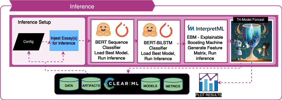
from torch.nn.functional import softmax
      
      
      essays_for_inference_final = pd.read_csv('/Users/lange/dev/ai-or-biology/data/train_drcat_04.csv')
      
      #essays_for_inference_final = pd.read_csv('/kaggle/input/llm-detect-ai-generated-text/test_essays.csv')
      essays_for_inference_1 = essays_for_inference_final[essays_for_inference_final['label'] == 1].sample(20)
      essays_for_inference_0 = essays_for_inference_final[essays_for_inference_final['label'] == 0].sample(20) #essays_for_inference[essays_for_inference['label'] == 0].sample(len(essays_for_inference_train))
      essays_for_inference_cntat = pd.concat([essays_for_inference_1, essays_for_inference_0])
      essays_for_inference_final = essays_for_inference_cntat.sample(frac=1).reset_index(drop=True)
      

Preprocesses Data

back stepping into the features pipeline for inference.

...

import joblib
      
      from sklearn.preprocessing import MinMaxScaler, StandardScaler
      import pandas as pd
      import traceback
      def scale_columns(df, columns_to_scale, scaler=None, scale_type='MinMaxScaler'):
          """
          Scale the specified columns in a DataFrame and add a suffix to the column names.
      
          Args:
              df (pandas.DataFrame): The DataFrame to scale.
              columns_to_scale (list): List of column names to scale.
              scaler (object, optional): Scaler object to use for scaling. If None, a new scaler object will be created.
              scale_type (str, optional): The type of scaler to use. Default is 'MinMaxScaler'. Options: 'MinMaxScaler', 'StandardScaler'.
      
          Returns:
              pandas.DataFrame: The full DataFrame with scaled columns added.
              pandas.DataFrame: A separate DataFrame with only the specified columns scaled.
              object: The scaler object used for scaling.
          """
          if scale_type == 'MinMaxScaler':
              scaler = MinMaxScaler() if scaler is None else scaler
          elif scale_type == 'StandardScaler':
              scaler = StandardScaler() if scaler is None else scaler
          else:
              raise ValueError("Invalid scale_type. Options: 'MinMaxScaler', 'StandardScaler'")
      
          scaled_columns = scaler.transform(df[columns_to_scale])
          scaled_df = pd.DataFrame(scaled_columns, columns=[col + '_scaled' for col in columns_to_scale])
      
          full_df = pd.concat([df.drop(columns=columns_to_scale), scaled_df], axis=1)
      
          return full_df, scaled_df, scaler
      
      def generate_features_for_inference(test_essays):
          try:
              #df_essays_copy = pd.read_pickle("scratch/df_essays_copy.pkl")
      
              ## Run them through the pipeline to get the features
              df_essays = pipeline_preprocess_text(test_essays)
              df_essays = process_readability_scores(df_essays)
              df_essays = process_semantic_density(df_essays)
              df_essays = process_semantic_flow_variability(df_essays)
              df_essays = apply_empath_analysis(df_essays)
              df_essays["textual_entropy"] = df_essays["text"].progress_apply(calculate_entropy)
              df_essays = process_syntactic_tree_patterns(df_essays)
      
              readability_columns = ['flesch_kincaid_grade', 'gunning_fog', 'coleman_liau_index', 'smog_index', 'ari', 'dale_chall', 'textual_entropy', 'semantic_density', 'semantic_flow_variability']
              scaler = joblib.load(f"{CFG.SCRATCH_PATH}/scaler_semantic_features.pkl")
              # Scale the columns using MinMaxScaler
              readability_scaled_backin_df, readability_scaled_df, readability_scaler = scale_columns(df_essays, readability_columns,scaler, scale_type='MinMaxScaler')
      
      
              psycho_columns = ['help','office','dance','money','wedding','domestic_work','sleep','medical_emergency','cold','hate','cheerfulness','aggression','occupation','envy','anticipation','family','vacation','crime','attractive','masculine','prison','health','pride','dispute','nervousness','government','weakness','horror','swearing_terms','leisure','suffering','royalty','wealthy','tourism','furniture','school','magic','beach','journalism','morning','banking','social_media','exercise','night','kill','blue_collar_job','art','ridicule','play','computer','college','optimism','stealing','real_estate','home','divine','sexual','fear','irritability','superhero','business','driving','pet','childish','cooking','exasperation','religion','hipster','internet','surprise','reading','worship','leader','independence','movement','body','noise','eating','medieval','zest','confusion','water','sports','death','healing','legend','heroic','celebration','restaurant','violence','programming','dominant_heirarchical','military','neglect','swimming','exotic','love','hiking','communication','hearing','order','sympathy','hygiene','weather','anonymity','trust','ancient','deception','fabric','air_travel','fight','dominant_personality','music','vehicle','politeness','toy','farming','meeting','war','speaking','listen','urban','shopping','disgust','fire','tool','phone','gain','sound','injury','sailing','rage','science','work','appearance','valuable','warmth','youth','sadness','fun','emotional','joy','affection','traveling','fashion','ugliness','lust','shame','torment','economics','anger','politics','ship','clothing','car','strength','technology','breaking','shape_and_size','power','white_collar_job','animal','party','terrorism','smell','disappointment','poor','plant','pain','beauty','timidity','philosophy','negotiate','negative_emotion','cleaning','messaging','competing','law','friends','payment','achievement','alcohol','liquid','feminine','weapon','children','monster','ocean','giving','contentment','writing','rural','positive_emotion','musical']
              # Scale the columns using MinMaxScaler
              scaler_psyco = joblib.load(f"{CFG.SCRATCH_PATH}/scaler_psycho_features.pkl")
              psycho_scaled_df_backin_df, psycho_scaled_df, psycho_scaler = scale_columns(df_essays, psycho_columns,scaler_psyco, scale_type='MinMaxScaler')
      
      
              # Define the columns to scale
              text_features = ['num_sentences', 'num_tokens', 'num_unique_lemmas', 'average_token_length', 'average_sentence_length', 'num_entities', 'num_noun_chunks', 'num_pos_tags', 'num_distinct_entities', 'average_entity_length', 'average_noun_chunk_length', 'max_depth', 'avg_branching_factor', 'total_nodes', 'total_leaves', 'unique_rules', 'tree_complexity', 'depth_variability']
              scaler_text = joblib.load(f"{CFG.SCRATCH_PATH}/scaler_tree_features.pkl")
              # Scale the columns using MinMaxScaler
              tree_feature_scaler_backin_df, tree_features_scaled_df, tree_feature_scaler = scale_columns(df_essays, 
                                                                                                          text_features,scaler_text, scale_type='MinMaxScaler')
      
      
              final_features_df = pd.concat([readability_scaled_df,tree_features_scaled_df,psycho_scaled_df], axis=1)
              #print(final_features_df.head())
              return final_features_df
              
      
          except Exception as e:
              # if any fail, revert to the bert inference
              print(f"Error in feature extraction: {e}")
              
      

Inference Functions

BERT-BiLSTM Classifier

import torch
      import pandas as pd
      
      
      def bert_inference(dataframe, model, tokenizer, max_length, device):
          """
          Performs inference on a dataframe using a pre-loaded model and returns softmax probabilities.
      
          Args:
          - dataframe (pd.DataFrame): DataFrame containing the texts to classify.
          - model (torch.nn.Module): Pre-loaded trained model for inference.
          - tokenizer (transformers.PreTrainedTokenizer): Tokenizer for the model.
          - max_length (int): Maximum sequence length for tokenization.
          - device (torch.device): The device to run the model on (CPU or GPU).
      
          Returns:
          - pd.DataFrame: Original DataFrame with additional columns for predictions and probabilities.
          """
          model.to(device)
          model.eval()
      
          predictions = []
          probabilities = []
      
          for _, row in dataframe.iterrows():
              text = row['text']
      
              inputs = tokenizer.encode_plus(
                  text,
                  add_special_tokens=True,
                  max_length=max_length,
                  padding='max_length',
                  truncation=True,
                  return_tensors='pt'
              )
      
              input_ids = inputs['input_ids'].to(device)
              attention_mask = inputs['attention_mask'].to(device)
      
              with torch.no_grad():
                  output = model(input_ids, attention_mask)
      
                  logits = output.logits if hasattr(output, 'logits') else output
      
                  probs = torch.nn.functional.softmax(logits, dim=1)
                  probabilities_ind = torch.nn.functional.softmax(probs, dim=1).cpu().numpy()[0]
      
                  prediction = torch.argmax(probs, dim=1).cpu().numpy()[0]
      
                  if (prediction>= 1):
                      probability = max(probabilities_ind)
                  else:
                      probability = min(probabilities_ind)
      
                  predictions.append(prediction)
                  probabilities.append(probability)
      
          dataframe['predicted_label'] = predictions
          dataframe['probability'] = probabilities
          return dataframe
      

EBM Explainable Boosting Machine

import pandas as pd
      import numpy as np
      from scipy.special import softmax
      
      def ebm_inference(model, data):
          """
          Performs inference using an EBM model and returns predictions with probabilities.
      
          Args:
          - model: Trained EBM model.
          - data (pd.DataFrame): DataFrame containing the data for inference.
      
          Returns:
          - pd.DataFrame: DataFrame with predictions and corresponding probabilities.
          """
      
          X = data.values
      
          # Initialize lists for predictions and probabilities
          predictions = []
          probabilities = []
      
          # Iterate over each row in the input data
          for i in range(len(X)):
              # Get the current row and reshape it
              row = X[i].reshape(1, -1)
      
              # Make prediction and calculate probabilities
              prediction = model.predict(row)
              probabilities_ind = model.predict_proba(row)
              softmax_probabilities = softmax(probabilities_ind, axis=1) # ebm prob is a sigmoid, we need softmax which extends sigmoid
      
              # Append the prediction and probability to the lists
              predictions.append(prediction[0])
              probabilities.append(softmax_probabilities[0][1])
      
          # Combine predictions and probabilities into a single DataFrame
          results = pd.DataFrame({
              'predicted_label': predictions,
              'probability': probabilities
          })
      
          return results
      

Clean Test Essays

df_to_classify = pipeline_preprocess_text(essays_for_inference_final)
      

100%|██████████| 40/40 [00:00<00:00, 205.28it/s]
      

Preprocessing completed in 0.20 seconds
      

⓶ Inference 🤗 BertForSequenceClassification

...

from transformers import BertTokenizer, BertForSequenceClassification, TrainingArguments
      import torch
      from torch import nn
      from transformers import BertModel
      
      #if(CFG.EBM_ONLY == False):
      import torch
      from torchsummary import summary
      # This is sloppy - but leaving for now asit works. Will clean up later.
      # Configuration and Usage
      device = torch.device("cuda" if torch.cuda.is_available() else "cpu")
      
      # Load the tokenizer, study, and best model
      
      
      import pickle
      with open(f'{CFG.SCRATCH_PATH}/bert_seq_class_tokeniser.pkl', 'rb') as f:
          tokenizer = pickle.load(f)
          
      with open(f'{CFG.SCRATCH_PATH}/bert_seq_class_study.pkl', 'rb') as f:
          study = pickle.load(f)
          
      model_config = {
      'bert_model': CFG.BERT_MODEL,
      'do_lower_case': False,
      'num_labels': 2,
      'output_attentions': False,
      'output_hidden_states': False,
      'max_length': 32,
      'optuna_trials': 1,
      'epochs': 1,
      'device': torch.device('cuda:0' if torch.cuda.is_available() else 'cpu')
      }
      
      # Copy of the args from the model. putting them here just in case it run wothout that cell. 
      training_args = TrainingArguments(
          output_dir=f'{CFG.SCRATCH_PATH}/results',
          num_train_epochs=model_config['epochs'],
          per_device_train_batch_size=16,
          per_device_eval_batch_size=32,
          warmup_steps=100,
          weight_decay=0.01,
          logging_dir=f'{CFG.SCRATCH_PATH}/logs/bert_sequence_classifier',
          learning_rate=5e-5,
          adam_epsilon=1e-8,
          do_train=True,
          do_eval=True,
          no_cuda=False,
          evaluation_strategy="epoch",
          save_strategy="steps",
          logging_steps=500,
          save_steps=500,
      )
      
      
      
      # Load the model
      ## Get params from the best trial
      #best_trial_params = study.best_trial.params
      
      # set the training arguments with the best trail values
      training_args.learning_rate = study["learning_rate"]
      training_args.per_device_train_batch_size = study["batch_size"]
      
      # load the model with the best OPTUNA trial
      best_model = BertClassifier(training_args, model_config)
      
      
      #best_model.model.load_state_dict(torch.load(f"{CFG.SCRATCH_PATH}/bert_sequence_classifier_best.pt"))
      best_model.model.load_state_dict(torch.load(f"{CFG.SCRATCH_PATH}/bert_sequence_classifier_best.pt",map_location=device))
      print("----- Bert For Sequence Classification -----")
      print(best_model.model)
      
      # Run Inference
      bert_seq_classifier_inference_results = bert_inference(df_to_classify, best_model.model, tokenizer,
                                                             model_config['max_length'], device)
      
      
      if(CFG.KAGGLE_RUN == False):
          correct_predictions = (bert_seq_classifier_inference_results['label'] == bert_seq_classifier_inference_results['predicted_label']).sum()
          # Calculate the total number of predictions
          total_predictions = len(bert_seq_classifier_inference_results)
      
          # Calculate the accuracy
          accuracy = correct_predictions / total_predictions
      
          # Print the statistics
          print(f"Total predictions: {total_predictions}")
          print(f"Correct predictions: {correct_predictions}")
          print(f"Accuracy: {accuracy}")
      
          # Get the true labels and predicted labels as numpy arrays
          true_labels = bert_seq_classifier_inference_results['label'].to_numpy()
          predicted_labels = bert_seq_classifier_inference_results['predicted_label'].to_numpy()
      
          # Calculate the confusion matrix
          cm = confusion_matrix(true_labels, predicted_labels)
      
          # Print the confusion matrix
          print("Confusion Matrix:")
          print(cm)
      
          incorrect_row_numbers = np.where(true_labels != predicted_labels)[0]
      
          # Print the row numbers of incorrect predictions
          print("Incorrect Row Numbers:")
          print(incorrect_row_numbers)
      

Some weights of BertForSequenceClassification were not initialized from the model checkpoint at bert-base-uncased and are newly initialized: ['classifier.bias', 'classifier.weight']
      You should probably TRAIN this model on a down-stream task to be able to use it for predictions and inference.
      

----- Bert For Sequence Classification -----
      BertForSequenceClassification(
        (bert): BertModel(
          (embeddings): BertEmbeddings(
            (word_embeddings): Embedding(30522, 768, padding_idx=0)
            (position_embeddings): Embedding(512, 768)
            (token_type_embeddings): Embedding(2, 768)
            (LayerNorm): LayerNorm((768,), eps=1e-12, elementwise_affine=True)
            (dropout): Dropout(p=0.1, inplace=False)
          )
          (encoder): BertEncoder(
            (layer): ModuleList(
              (0-11): 12 x BertLayer(
                (attention): BertAttention(
                  (self): BertSelfAttention(
                    (query): Linear(in_features=768, out_features=768, bias=True)
                    (key): Linear(in_features=768, out_features=768, bias=True)
                    (value): Linear(in_features=768, out_features=768, bias=True)
                    (dropout): Dropout(p=0.1, inplace=False)
                  )
                  (output): BertSelfOutput(
                    (dense): Linear(in_features=768, out_features=768, bias=True)
                    (LayerNorm): LayerNorm((768,), eps=1e-12, elementwise_affine=True)
                    (dropout): Dropout(p=0.1, inplace=False)
                  )
                )
                (intermediate): BertIntermediate(
                  (dense): Linear(in_features=768, out_features=3072, bias=True)
                  (intermediate_act_fn): GELUActivation()
                )
                (output): BertOutput(
                  (dense): Linear(in_features=3072, out_features=768, bias=True)
                  (LayerNorm): LayerNorm((768,), eps=1e-12, elementwise_affine=True)
                  (dropout): Dropout(p=0.1, inplace=False)
                )
              )
            )
          )
          (pooler): BertPooler(
            (dense): Linear(in_features=768, out_features=768, bias=True)
            (activation): Tanh()
          )
        )
        (dropout): Dropout(p=0.1, inplace=False)
        (classifier): Linear(in_features=768, out_features=2, bias=True)
      )
      Total predictions: 40
      Correct predictions: 38
      Accuracy: 0.95
      Confusion Matrix:
      [[20  0]
       [ 2 18]]
      Incorrect Row Numbers:
      [ 1 24]
      

⓷ Inference - 🤗 BERT-BiLSTM Classifier

...

model_config = {
          'bert_model_name': CFG.BERT_MODEL,
          'num_classes': 2,
          'max_length': 128,
          'batch_size': 16,
          'num_epochs': 4,
          'train_data': df_essays_copy,
          'num_trials': 2,
      }
      
      
      # Pickle the tokenizer, study, and best model
      with open(f'{CFG.SCRATCH_PATH}/custom_bert_tokenizer.pkl', 'rb') as f:
          tokenizer = pickle.load(f)
      
      with open(f'{CFG.SCRATCH_PATH}/best_custom_model_study.pkl', 'rb') as f:
          study = pickle.load(f)
      
      
          # Retrain model with best hyperparameters
      best_trial = study.best_trial
      
      #Load the model with the best trial
      best_trial_params = study.best_trial.params
      learning_rate = best_trial_params["learning_rate"]
      dropout_rate = best_trial_params["dropout_rate"]
      fc_layer_size = best_trial_params["fc_layer_size"]
      lstm_hidden_size = best_trial_params["lstm_hidden_size"]
      lstm_layers = best_trial_params["lstm_layers"]
      
      best_model = BERTBiLSTMClassifier(model_config['bert_model_name'], model_config['num_classes'], dropout_rate, fc_layer_size,lstm_layers)
      best_model.load_state_dict(torch.load(f'{CFG.SCRATCH_PATH}/bert_finetune_custom_best.pt',map_location=device))
      #Initialize the best model with the optimal hyperparameters
      best_model.to(device)
      
      print(best_model)
      custom_bert_inference_results = bert_inference(df_to_classify, best_model, tokenizer, model_config['max_length'], device)
      
      if(CFG.KAGGLE_RUN == False):
          ## STATISTICS
          #Calculate the number of correct predictions
          correct_predictions = (custom_bert_inference_results['label'] == custom_bert_inference_results['predicted_label']).sum()
          # Calculate the total number of predictions
          total_predictions = len(custom_bert_inference_results)
      
          # Calculate the accuracy
          accuracy = correct_predictions / total_predictions
      
          # Print the statistics
          print(f"Total predictions: {total_predictions}")
          print(f"Correct predictions: {correct_predictions}")
          print(f"Accuracy: {accuracy}")
      
          # Get the true labels and predicted labels as numpy arrays
          true_labels = custom_bert_inference_results['label'].to_numpy()
          predicted_labels = custom_bert_inference_results['predicted_label'].to_numpy()
      
          # Calculate the confusion matrix
          cm = confusion_matrix(true_labels, predicted_labels)
          if(CFG.CLEARML_ON):
              clearml_bertmodel_custom.log_data(data=cm,title='Custom Bert Classifier Inference Results Confusoon Matric')
          # Print the confusion matrix
          print("Confusion Matrix:")
          print(cm)
      
          incorrect_row_numbers = np.where(true_labels != predicted_labels)[0]
      
          # Print the row numbers of incorrect predictions
          print("Incorrect Row Numbers:")
          print(incorrect_row_numbers)
      

BERTBiLSTMClassifier(
        (bert): BertModel(
          (embeddings): BertEmbeddings(
            (word_embeddings): Embedding(30522, 768, padding_idx=0)
            (position_embeddings): Embedding(512, 768)
            (token_type_embeddings): Embedding(2, 768)
            (LayerNorm): LayerNorm((768,), eps=1e-12, elementwise_affine=True)
            (dropout): Dropout(p=0.1, inplace=False)
          )
          (encoder): BertEncoder(
            (layer): ModuleList(
              (0-11): 12 x BertLayer(
                (attention): BertAttention(
                  (self): BertSelfAttention(
                    (query): Linear(in_features=768, out_features=768, bias=True)
                    (key): Linear(in_features=768, out_features=768, bias=True)
                    (value): Linear(in_features=768, out_features=768, bias=True)
                    (dropout): Dropout(p=0.1, inplace=False)
                  )
                  (output): BertSelfOutput(
                    (dense): Linear(in_features=768, out_features=768, bias=True)
                    (LayerNorm): LayerNorm((768,), eps=1e-12, elementwise_affine=True)
                    (dropout): Dropout(p=0.1, inplace=False)
                  )
                )
                (intermediate): BertIntermediate(
                  (dense): Linear(in_features=768, out_features=3072, bias=True)
                  (intermediate_act_fn): GELUActivation()
                )
                (output): BertOutput(
                  (dense): Linear(in_features=3072, out_features=768, bias=True)
                  (LayerNorm): LayerNorm((768,), eps=1e-12, elementwise_affine=True)
                  (dropout): Dropout(p=0.1, inplace=False)
                )
              )
            )
          )
          (pooler): BertPooler(
            (dense): Linear(in_features=768, out_features=768, bias=True)
            (activation): Tanh()
          )
        )
        (lstm): LSTM(768, 32, num_layers=3, batch_first=True, bidirectional=True)
        (dropout): Dropout(p=0.0456841451290286, inplace=False)
        (fc): Linear(in_features=64, out_features=2, bias=True)
        (relu): ReLU()
      )
      Total predictions: 40
      Correct predictions: 39
      Accuracy: 0.975
      Confusion Matrix:
      [[20  0]
       [ 1 19]]
      Incorrect Row Numbers:
      [1]
      

⓸ Inference - 🔬 EBM | Explainable Boosting Classifier

...

import pandas as pd
      import numpy as np
      from interpret.glassbox import ExplainableBoostingClassifier
      from scipy.special import softmax
      
      
      # This creates all the features for each text field in the dataframe.
      essays_for_inference_sample = generate_features_for_inference(df_to_classify)
      
      # create our features df with the columns named correctly
      features = pd.DataFrame(essays_for_inference_sample, columns=essays_for_inference_sample.columns)
      
      # Set logging level to ERROR
      logging.getLogger('interpret').setLevel(logging.ERROR)
      
      # with open(f'{CFG.SCRATCH_PATH}/ebm.pkl', 'rb') as f:
      #     ebm = ebm.load(f)
      ## Get yout goods and bads          
      ebm_inference_results = ebm_inference(ebm_gs, features)
      
      if(CFG.CLEARML_ON):
          clearml_ebm.log_data(data=features,title='Explainable Boosting Model Inference Data')
          clearml_ebm.log_data(data=ebm_inference_results,title='Explainable Boosting Model Inference Results')
      ## Output the model stats 
      
      if(CFG.KAGGLE_RUN == False):
          labels_df = df_to_classify['label']
          correct_predictions = (df_to_classify['label'].reset_index(drop=True) == ebm_inference_results['predicted_label'].reset_index(drop=True)).sum()
          # Calculate the total number of predictions
          total_predictions = len(ebm_inference_results)
      
          # Calculate the accuracy
          accuracy = correct_predictions / total_predictions
      
          # Print the statistics
          print(f"Total predictions: {total_predictions}")
          print(f"Correct predictions: {correct_predictions}")
          print(f"Accuracy: {accuracy}")
      
          # Get the true labels and predicted labels as numpy arrays
          true_labels = df_to_classify['label'].to_numpy()
          predicted_labels = ebm_inference_results['predicted_label'].to_numpy()
      
          # Calculate the confusion matrix
          cm = confusion_matrix(true_labels, predicted_labels)
      
          # Print the confusion matrix
          print("Confusion Matrix:")
          print(cm)
      
          incorrect_row_numbers = np.where(true_labels != predicted_labels)[0]
      
          # Print the row numbers of incorrect predictions
          print("Incorrect Row Numbers:")
          print(incorrect_row_numbers)
      

100%|██████████| 40/40 [00:00<00:00, 247.12it/s]
      

Preprocessing completed in 0.16 seconds
      

Total predictions: 40
      Correct predictions: 35
      Accuracy: 0.875
      Confusion Matrix:
      [[18  2]
       [ 3 17]]
      Incorrect Row Numbers:
      [ 1 11 27 29 36]
      

EBM Performance

if(CFG.KAGGLE_RUN == False):
          from interpret.perf import ROC
      
          ebm_perf = ROC(ebm.predict_proba).explain_perf(X_test, y_test, name='EBM')
          show(ebm_perf)
      

⓹ Ensemble Scoring

...

      if(CFG.ENSAMBLE_STRATEGY == 1): # For three models
          majority_label = (bert_seq_classifier_inference_results['predicted_label'] + 
                          custom_bert_inference_results['predicted_label'] + 
                          ebm_inference_results['predicted_label']).apply(lambda x: 1 if x >= 1 else 0)
      
      
          average_probability = (bert_seq_classifier_inference_results['probability'] + 
                              custom_bert_inference_results['probability'] + 
                              ebm_inference_results['probability']) / 3
      
      if(CFG.ENSAMBLE_STRATEGY == 2): # For 2 models - best one
          majority_label = (#bert_seq_classifier_inference_results['predicted_label'] + 
                          custom_bert_inference_results['predicted_label'] + 
                          ebm_inference_results['predicted_label']).apply(lambda x: 1 if x >= 1 else 0)
      
      
          average_probability = (#bert_seq_classifier_inference_results['probability'] + 
                              custom_bert_inference_results['probability'] + 
                              ebm_inference_results['probability']) / 2
      # Final Decision: If labels agree, use them. If not, use average probability.
      # Ensamble AVG strat 1
      
      # =================
      # CFG.ENSAMBLE_STRATEGY 1
      if(CFG.ENSAMBLE_STRATEGY == 1):
          final_decision = majority_label.copy()
          for i in range(len(bert_seq_classifier_inference_results)):
              if ebm_inference_results['predicted_label'][i] != custom_bert_inference_results['predicted_label'][i]: # Best Models Disagree
                  final_decision[i] = 1 if average_probability[i] >= 0.50 else 0  
      
       # =================
      # CFG.ENSAMBLE_STRATEGY 2        
      if(CFG.ENSAMBLE_STRATEGY == 2):
          final_decision = majority_label.copy()
          for i in range(len(bert_seq_classifier_inference_results)):
              if ebm_inference_results['predicted_label'][i] != custom_bert_inference_results['predicted_label'][i]: # Best Models Disagree
                  final_decision[i] = 1 if average_probability[i] >= 0.50 else 0   
      
      
      ensemble_results = pd.DataFrame({
              'final_predicted_label': final_decision,
              #'label': custom_bert_inference_results['label'],
              'average_probability': average_probability,
              #'source': custom_bert_inference_results['source'],
              'text': custom_bert_inference_results['text']
          })
          
      
      
      if(CFG.CLEARML_ON):
          clearml_ebm.log_data(data=ensemble_results,title='Exsemble Model Scoring Results')
      
      if(CFG.KAGGLE_RUN == False):
      
          ## Ensamble ------------------------
          correct_predictions = (df_to_classify['label'].reset_index(drop=True) == 
                              ensemble_results['final_predicted_label'].reset_index(drop=True)).sum()
          # Calculate the total number of predictions
          total_predictions = len(ensemble_results)
      
          # Calculate the accuracy
          accuracy = correct_predictions / total_predictions
      
          # Print the statistics
          print(f"Total predictions: {total_predictions}")
          print(f"Correct predictions: {correct_predictions}")
          print(f"Accuracy: {accuracy}")
      
          # Get the true labels and predicted labels as numpy arrays
          true_labels = df_to_classify['label'].to_numpy()
          predicted_labels = ensemble_results['final_predicted_label'].to_numpy()
          predicted_averages = ensemble_results['average_probability'].to_numpy()
      
          # Calculate the confusion matrix
          cm = confusion_matrix(true_labels, predicted_labels)
          if(CFG.CLEARML_ON):
              clearml_ebm.log_data(data=cm,title='Exsemble Model Scoring Results Confusoon Matric')
      
          # Print the confusion matrix
          print("Confusion Matrix:")
          print(cm)
      
      
          incorrect_row_numbers = np.where(true_labels != predicted_labels)[0]
      
          # Print the row numbers of incorrect predictions
          print("Incorrect Row Numbers:")
          print(incorrect_row_numbers)
          print(predicted_averages)
      

Total predictions: 40
      Correct predictions: 38
      Accuracy: 0.95
      Confusion Matrix:
      [[19  1]
       [ 1 19]]
      Incorrect Row Numbers:
      [ 1 36]
      [0.69439393 0.33834966 0.70149138 0.7054628  0.3089722  0.70524129
       0.31124632 0.308972   0.31014631 0.30891109 0.65973125 0.4364831
       0.31098962 0.7054017  0.31575136 0.69931882 0.3998628  0.69748983
       0.70319676 0.30904756 0.30995664 0.3093674  0.31151034 0.7049542
       0.70468167 0.68598632 0.70542308 0.51682635 0.30910718 0.58167151
       0.30929284 0.30888784 0.70514635 0.69362241 0.30898159 0.311092
       0.5090657  0.70544873 0.70528596 0.30920638]
      

# print(bert_seq_classifier_inference_results['probability'])
      # print(custom_bert_inference_results['probability'])
      # print(ebm_inference_results['probability'])
      

☯️ Predictions

🎙 References

Relating Natural Language Aptitude to Individual Differences in Learning Programming Languages) [1]

@article{article,
        author = {Prat, Chantel and Madhyastha, Tara and Mottarella, Malayka and Kuo, Chu-Hsuan},
        year = {2020},
        month = {03},
        pages = {},
        title = {Relating Natural Language Aptitude to Individual Differences in Learning Programming Languages},
        volume = {10},
        journal = {Scientific Reports},
        doi = {10.1038/s41598-020-60661-8}
      }
          
      

InterpretML: A Unified Framework for Machine Learning Interpretability" (H. Nori, S. Jenkins, P. Koch, and R. Caruana 2019)[2]

@article{nori2019interpretml,
        title={InterpretML: A Unified Framework for Machine Learning Interpretability},
        author={Nori, Harsha and Jenkins, Samuel and Koch, Paul and Caruana, Rich},
        journal={arXiv preprint arXiv:1909.09223},
        year={2019}
      }
          
      

The Psychological Meaning of Words: LIWC and Computerized Text Analysis Methods[3]

@article{article,
          author = {Tausczik, Yla and Pennebaker, James},
          year = {2010},
          month = {03},
          pages = {24-54},
          title = {The Psychological Meaning of Words: LIWC and Computerized Text Analysis Methods},
          volume = {29},
          journal = {Journal of Language and Social Psychology},
          doi = {10.1177/0261927X09351676}
      }
          
      

“Attention is all you need” (Vaswani, Ashish & Shazeer, Noam & Parmar, Niki & Uszkoreit, Jakob & Jones, Llion & Gomez, Aidan & Kaiser, Lukasz & Polosukhin, Illia. (2017)) [4]

@misc{vaswani2023attention,
            title={Attention Is All You Need}, 
            author={Ashish Vaswani and Noam Shazeer and Niki Parmar and Jakob Uszkoreit and Llion Jones and Aidan N. Gomez and Lukasz Kaiser and Illia Polosukhin},
            year={2023},
            eprint={1706.03762},
            archivePrefix={arXiv},
            primaryClass={cs.CL}
      }
          
      

Proceedings of the 57th Annual Meeting of the Association for Computational Linguistics[5]

@inproceedings{kitaev-etal-2019-multilingual,
          title = "Multilingual Constituency Parsing with Self-Attention and Pre-Training",
          author = "Kitaev, Nikita  and
            Cao, Steven  and
            Klein, Dan",
          booktitle = "Proceedings of the 57th Annual Meeting of the Association for Computational Linguistics",
          month = jul,
          year = "2019",
          address = "Florence, Italy",
          publisher = "Association for Computational Linguistics",
          url = "https://www.aclweb.org/anthology/P19-1340",
          doi = "10.18653/v1/P19-1340",
          pages = "3499--3505",
      }
          
      

Constituency Parsing with a Self-Attentive Encoder[6]

@inproceedings{kitaev-klein-2018-constituency,
          title = "Constituency Parsing with a Self-Attentive Encoder",
          author = "Kitaev, Nikita  and
            Klein, Dan",
          booktitle = "Proceedings of the 56th Annual Meeting of the Association for Computational Linguistics (Volume 1: Long Papers)",
          month = jul,
          year = "2018",
          address = "Melbourne, Australia",
          publisher = "Association for Computational Linguistics",
          url = "https://www.aclweb.org/anthology/P18-1249",
          doi = "10.18653/v1/P18-1249",
          pages = "2676--2686",
      }
          
      

Other Stuff

# #  # End the timer
      # # end_time = time.time()
      
      # # # Calculate the total execution time
      # # total_time = end_time - start_time
      
      # print(f"Total execution time: {total_time} seconds")
      # print(f"Total execution time: {total_time/60} minues")
      # print(f"Total execution time: {total_time/60/60} hours")
      
      
      # ## Stats - source GPT4
      # #  # End the timer
      # # end_time = time.time()
      
      # # # Calculate the total execution time
      # # total_time = end_time - start_time
      # import psutil
      
      # # Get CPU information
      # #cpu_info = psutil.cpu_freq()
      # cpu_percent = psutil.cpu_percent()
      
      # # Get memory information
      # memory_info = psutil.virtual_memory()
      
      # # Get disk usage information
      # disk_usage = psutil.disk_usage('/')
      
      # # Print the hardware and software specifications
      # #print("CPU Frequency:", cpu_info.current, "MHz")
      
      # print("Total Memory:", memory_info.total // (1024 ** 3), "GB")
      # print("Disk Usage:", disk_usage.used // (1024 ** 3), "GB")
      
      # # get device
      # device = torch.device("cuda" if torch.cuda.is_available() else "cpu")
      # print("cuda? :", device)
      

Readability and Semantic Features

for more insight on our features

# labels = df_essays_copy['label'].tolist()
      # features = readability_scaled_df #psycho_scaled_df
      # X_train, X_test, y_train, y_test = train_test_split(features, labels, test_size=0.2, random_state=42)
      
      # ebm = ExplainableBoostingClassifier(interactions=0, 
      #                                     feature_names=features.columns.tolist())
      
      # ebm.fit(X_train, y_train)
      # ebm.score(X_test, y_test)
      
      # from interpret import show
      
      # ebm_global = ebm.explain_global()
      # show(ebm_global)
      
      # ebm_local = ebm.explain_local(X_test, y_test)
      # show(ebm_local)
      

Psycholinguistic Features

# labels = df_essays_copy['label'].tolist()
      # features = psycho_scaled_df #psycho_scaled_df
      # X_train, X_test, y_train, y_test = train_test_split(features, labels, test_size=0.2, random_state=42)
      
      # ebm = ExplainableBoostingClassifier(interactions=0, 
      #                                     feature_names=features.columns.tolist())
      
      
      # ebm.fit(X_train, y_train)
      # ebm.score(X_test, y_test)
      
      # from interpret import show
      
      # ebm_global = ebm.explain_global()
      # show(ebm_global)
      
      # ebm_local = ebm.explain_local(X_test, y_test)
      # show(ebm_local)
      

Tree Features and Stats

# labels = df_essays_copy['label'].tolist()
      # features = tree_features_scaled_df #psycho_scaled_df
      # X_train, X_test, y_train, y_test = train_test_split(features, labels, test_size=0.2, random_state=42)
      
      # ebm = ExplainableBoostingClassifier(interactions=0, 
      #                                     feature_names=features.columns.tolist())
      
      
      # ebm.fit(X_train, y_train)
      # ebm.score(X_test, y_test)
      
      # from interpret import show
      
      # ebm_global = ebm.explain_global()
      # show(ebm_global)
      
      # ebm_local = ebm.explain_local(X_test, y_test)
      # show(ebm_local)
      

# categories_to_plot = ['average_token_length','num_pos_tags','num_distinct_entities','average_entity_length','average_noun_chunk_length','max_depth','avg_branching_factor','total_nodes','total_leaves','unique_rules','tree_complexity','depth_variability']
      
      
      # if(CFG.CLEARML_ON):
      #     plot_categories_box(df_essays, categories_to_plot,clearml_handler.task)
      # else:
      #     plot_categories_box(df_essays, categories_to_plot)