
Unsexy Series Overview
Not everyone gets to retrain the GPT-2 model to generate droll poetry 21, or tell fart jokes. Some of us need to build working solutions with disparate data that solve real business problems.
We'll cover some of the more important yet rarely discussed topics of applied Data Science in this little vignette of presentations. Starting with Dealing with Imbalanced Data.
Don't get me wrong — I'm re-tuning the GPT-2 Grover-Mega with every word George Carlin has ever written or said. Along with a bunch of other brilliant comedians. FunnyBot will take form. In the meantime, we all have to make a living.
The Data
I will be using two years (8 quarters) of data from https://www.fanniemae.com/portal/funding-the-market/data/loan-performance-data.html.
I'm using the Single-Family Fixed Rate Mortgage Dataset 2016-2017:
Fannie Mae provides both an acquisitions file and a performance file for loans within its Single-Family Loan Performance Dataset. On a quarterly basis, the dataset is updated to add another quarter of acquisitions and another quarter of performance.
What's so interesting about this data?
- First of all it's massive. There are ~500K rows of acquisitions per quarter from a bevy of origination sources. So by choosing only two years you get ~4Million rows of unique acquisition data along with the date of foreclosure if it exists.
- We can focus on short term risk for secondary markets. Most mortgage lending/trading/purchasing schemes today focused on the first two or three years of the note.
- It contains information that has yet to be labeled. I use 2016-2017 only so there is a lot of data without a foreclosure date even though one may exist in 2018-2019. This is perfect for out-of-sample validation and opens the window to re-weight or Transfer Learn for short term risk year after year.
- There are only 24 columns of very generic information that any company who buys or sells Mortgages can plugin and get highly accurate forecasts (according to my study below)
- It's the housing market + consumer credit risk. Who dosen't want this forecast?
- Mortgages are the most important consumer loan banks provide.
- I have love/hate relationship with folks who deal in this industry. I guess that makes it interesting to me.
First Things First
from sklearn.ensemble import RandomForestClassifier, RandomForestRegressor
from sklearn.model_selection import train_test_split
# sklearn preprocessing for dealing with categorical variables - we may do more but let's see..
from sklearn.preprocessing import LabelEncoder
## postgres goodies
from sqlalchemy import create_engine
import psycopg2
#IO :)
import io
## Gotta plot
import matplotlib.pyplot as plt
%matplotlib inline
## Just all around fun
from beakerx import *
# File system manangement
import os
## math
import numpy as np
# Duh
import pandas as pd
# Suppress warnings
import warnings
warnings.filterwarnings('ignore')
# matplotlib and seaborn for basic plotting
import matplotlib.pyplot as plt
import seaborn as sns
# To look at aquisition data to see what we're dealing with directly from the source.
import camelot
from camelot.core import Table, TableList
from imblearn.combine import SMOTEENN # for our unbalnaced data - see Citations at the bottom for more info
## This is the library we will use to explore the data and fit an interpretable model.
# No Black Boxes here. We want to know what's up at a per-forecast level.
# More on this library when we get to it.
from interpret.provider import InlineProvider
from interpret import set_visualize_provider
set_visualize_provider(InlineProvider())
Column Descriptions
Just to provide bit more insight before we get going, let's look at the data I'm working with.
- This is a PDF from their site. It's public, so they should not mind.
## With Camelot you can pull anything you want from a pdf. Here we're just converting the first tabular section into a DataFrame
import camelot
from camelot.core import Table, TableList
tables = camelot.read_pdf('https://loanperformancedata.fanniemae.com/lppub-docs/FNMA_SF_Loan_Performance_File_layout.pdf')
tables[0].df
Pre-Prosessing
What I have already done. And what you would need to do to replicate this model.
- The only piece of information that I pulled from the Performance data file is the Foreclosure Date, if one existed for that loan. Why? We don't want to do calculations on any performance information since at the time of origination that data was not available to the bank. You almost always want to reduce the complexity needed to create an accurate forecast. KISS.
- I merged the 16 text files on the loanid (8 quarters of Acquisition and Performance data) removing duplicate performance data.
- While merging I created a Label column that is a binary field based on whether that loanid was foreclosed using the foreclosure_date. So Simple.
- Why not take the date of foreclosure and length of the loan before they foreclosed into account? Again, not available at time of origination. We want generic as possible.
- I split origination dates into month and year. Why not?
- Dumped it all into posgres for easier analysis
Impute missing data with a simple 0 where fields were empty. The only row with (more than 1%) data missing was co_borrower_credit_score. But as you'll see, that's an important column in the model. If one exists, it a very telling piece of information. Actually it was the only row with missing data.
So in the end, i have a single table with the following information. note Label is our binary target.
[ "id", "channel", "seller", "interest_rate", "balance", "loan_term", "origination_date", "first_payment_date", "ltv", "cltv", "borrower_count", "dti", "borrower_credit_score", "first_time_homebuyer", "loan_purpose", "property_type", "unit_count", "occupancy_status", "property_state", "zip", "insurance_percentage", "product_type", "co_borrower_credit_score", "mortgage_insurance_type", "relocation_mortgage_indicator", "Label" ]
Load Data
# // psql conn
def create_connection():
engine = create_engine(
"postgresql+psycopg2://postgres:1234@0.0.0.0:5432/postgres"
)
conn = engine.raw_connection()
return conn
## Verify Connection
connection = create_connection()
cursor = connection.cursor()
print(connection.get_dsn_parameters(), "\n")
cursor.execute("SELECT version();")
record = cursor.fetchone()
print("You are connected to - ", record, "\n")
## Pull our dataframe - during preprossing I created a few psql tables, the latest data is in fork_data_chk2
df = pd.read_sql_query("""SELECT * FROM fork_data_chk2;""", create_connection())
df
Check for Missing Data
I'm pretty sure there is none after a few rounds of munging. But you can never be too safe. And we may want to kill some arbitrary columns. let's see.
plt.figure(figsize=(15, 20))
plt.subplot(231)
sns.heatmap(
pd.DataFrame(df.isnull().sum() / df.shape[0] * 100),
annot=True,
cmap=sns.color_palette("cool"),
linewidth=1,
linecolor="white",
)
plt.show()

Remember, for a commercial model we only want to use inputs that every lender will have access to at the time of origination.
- We should also drop Channel and Seller as they ended up being too important. Yes, there is such a thing. It can lead to curve fitting your model with ancillary data. But we don't know that yet. So we won't for the purpose of this demonstration.
## Kill some obvious unnessecary Data.
def do_drops():
# drop the nonsence
df.drop(["index"],axis=1, inplace=True)
df.drop(["Unnamed: 0"],axis=1, inplace=True)
df.drop(["id"],axis=1, inplace=True)
## We'll keep the Id's just in case we made a mistake of some kind
do_drops()
What Imbalanced data looks like
Does not get much clearer than this
## Holy crap is right
sns.countplot(df['Label'])

### let't get a count of 1,s in the Label column. I.e., The count of forclosures in our dataset.
df.query("Label == True")
How is this Imbalanced?
- Do the math, .03% of the 4 Million acquisitions have defaulted in the 2-year sample period. We could fix this by looking at a larger sample say 2000-2019 data. But we're not. We are going to make even the data at hand. Sometimes you just don't get more data and have to make use with what you've got.
Think they found the Higgs on actual collider data? Nope. Most HEP models are based on simulated data (derived from observational data, of course). Obviously, one must check ground truth in the end, as they did. I may do a HEP study in this series and you'll get to learn about Monte Carlo techniques and how to use Graph Convolution Networks for noise reduction. When dealing with collider data, the number one task in to filter the noise as there is there is a tremendous amount of it. But that's pretty sexy data science, and may not work here. We'll stick with the boring stuff.
Back to the task at hand
Rebalance the data
Ok, so we have WAY more 0,s than 1's. Happens all the time. Remember, data on the screen is just a derivative of truth. At least in this case it is. And it can be transformed back and forth in a million different ways.
There are common and trusted techniques used to re balance data. Some are listed below.
Re-sampling techniques are can be divided as such 19:
- Under-sampling the majority class(es).
- Over-sampling the minority class.
- Combining over- and under-sampling.
- Create ensemble balanced sets.
Under-sampling
- Random majority under-sampling with replacement
- Extraction of majority-minority Tomek links [1]1
- Under-sampling with Cluster Centroids
- NearMiss-(1 & 2 & 3) 2
- Condensed Nearest Neighbour 3
- One-Sided Selection 4
- Neighboorhood Cleaning Rule5
- Edited Nearest Neighbours 6
- Instance Hardness Threshold 7
- Repeated Edited Nearest Neighbours 14
- AllKNN 14
Over-sampling
- Random minority over-sampling with replacement
- SMOTE - Synthetic Minority Over-sampling Technique 8
- SMOTENC - SMOTE for Nominal Continuous8
- bSMOTE(1 & 2) - Borderline SMOTE of types 1 and 2 9
- SVM SMOTE - Support Vectors SMOTE 10
- ADASYN - Adaptive synthetic sampling approach for imbalanced learning 15
- KMeans-SMOTE 17
Over-sampling followed by under-sampling
Over-sampling followed by under-sampling
We are going to use the Synthetic Minority Oversampling Technique (SMOTE). Rather than simply oversampling the the minority class or undersampling the dominant class, we can actually do both simultaneously while creating “new” instances of the minority class. This will give us an even balance of 1's and 0's on the dataset.
A Quick EDA - Enter InterpretML
- eda = Exploratory Data Analysis
https://github.com/interpretml/interpret
InterpretML 20 is an open-source package for training interpretable machine learning models and explaining blackbox systems. Interpretability is essential for:
- Model debugging - Why did my model make this mistake?
- Detecting bias - Does my model discriminate?
- Human-AI cooperation - How can I understand and trust the model's decisions?
- Regulatory compliance - Does my model satisfy legal requirements?
- High-risk applications - Healthcare, finance, judicial, ...
I think machine learning has progressed to a point where you have to explain yourself at a granular level. With each forecast you should know WHY and HOW it was derived. Or you have a dumb model. Do you or you or your managers still wonder how each forecast is made?
As the engineers of Interpret eloquently put it
If a tree fell in your random forest, would anyone notice?
Microsoft Research has developed an algorithm called the Explainable Boosting Machine (EBM) which has both high accuracy and interpretability. EBM uses modern machine learning techniques like bagging and boosting to breathe new life into traditional GAMs (Generalized Additive Models). This makes them as accurate as random forests and gradient boosted trees, and also enhances their intelligibility and editability20.
EBM is a fast implementation of GA2M.
\begin{equation}g(E[y])=\beta_{0}+\sum f_{j}\left(x_{j}\right)\end{equation}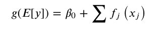
The EBM has a few major improvements over traditional GAMs
- First, EBM learns each feature function fj using modern machine learning techniques such as bagging and gradient boosting. The boosting procedure is carefully restricted to train on one feature at a time in round-robin fashion using a very low learning rate so that feature order does not matter. It round-robin cycles through features to mitigate the effects of co-linearity and to learn the best feature function fj for each feature to show how each feature contributes to the model’s prediction for the problem.
- Second, EBM can automatically detect and include pairwise interaction terms of the form (the key to it's sucess):
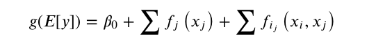
- In addition to EBM, InterpretML also supports methods like LIME, SHAP, linear models, partial dependence, decision trees and rule lists. The package makes it easy to compare and contrast models to find the best one for your needs.
We're going to use a tiny piece of its capabilities. So be sure to investigate on your own
Prepare for battle
## You've done this a million times
from sklearn.model_selection import train_test_split
train_cols = df.columns[0:-1]
label = df.columns[-1:]
X = df[train_cols]
y = df[label]
seed = 1
X_train, X_test, y_train, y_test = train_test_split(
X, y, test_size=0.20, random_state=seed
)
Explore the dataset
As you'll see this is a recipe for a biased model.
Check out each feature and click on the [0 Blue] Box on the chart to see only the 1's (foreclosures). And it's quite uniform for each feature. To me this says, while the training data is very unbalanced, the ground truth in and of itself NOT. But for a proper unbiased forecast, we have to balance our data for the algo.
Take a close look at both the 1 and 0 of dti (debt to income),Borrower Credit Score, Interest Rate and LTV (original Loan to Value)
Even if you knew nothing of credit or mortgages, the data clearly shows these will be the deciding factors.
And we'll have to make sure our re balanced data set represents this. It does, but still, keep that in mind when doing any type of re sampling. HAVE A GROUND TRUTH REFERENCE!
from interpret import show
from interpret.data import ClassHistogram
hist = ClassHistogram().explain_data(X_train, y_train, name = 'Train Data')
show(hist)
First Let's make everything a number. https://scikit-learn.org/stable/modules/generated/sklearn.preprocessing.OrdinalEncoder.html
This treats all columns as categorical information. Are they all? No. Is it the right thing to do? For classification of this kind..Maybe. Let's find out.
This is why I love Science. It's all trial and error based on what you think may work. Then try your damnedest to prove yourself wrong. And when you think you're right, others will try to prove you wrong even harder. Not a bad system.
"Pass on what you have learned. Strength, mastery, hmm… but weakness, folly, failure also. Yes: failure, most of all. The greatest teacher, failure is. Luke, we are what they grow beyond. That is the true burden of all masters" - Yoda 23
headers = list(df.columns.values) ## we'll put these back on after we ecode
from sklearn.preprocessing import OrdinalEncoder
def prepare_inputs(ds):
oe = OrdinalEncoder()
oe.fit(ds)
ds = oe.transform(ds)
return ds
## back to dataframe and add our headers
df = prepare_inputs(df)
df_new = pd.DataFrame(data=df, columns=headers)
df_new
SMOTE - the whole point of this notebook.
We're resampling 4 Million rows of data. This could take a while. Precicely 2hrs and 22 minutes on my very fast machine.
Better yet. As this whole excersise is basically the next 5 lines of code. Deep Dive.
- We first resample the data. I.,e., balance it. using SMOTE 24
- Then we DataFrame our output (Numpy Arrays)
- And slap the header row back on, to continue proper EDA.
from imblearn.combine import SMOTEENN
sm = SMOTEENN()
y = df_new['Label'].values
X = df_new.drop(['Label'], axis=1).values
X_resampled, y_resampled = sm.fit_sample(X, y)
DataFrame it and put header row back on resampled data.
# train_cols = df_new.columns[0:-1]
# train_cols
df_new_x = pd.DataFrame(data=X_resampled, columns=[
"channel",
"seller",
"interest_rate",
"balance",
"loan_term",
"origination_date",
"first_payment_date",
"ltv",
"cltv",
"borrower_count",
"dti",
"borrower_credit_score",
"first_time_homebuyer",
"loan_purpose",
"property_type",
"unit_count",
"occupancy_status",
"property_state",
"zip",
"insurance_percentage",
"product_type",
"co_borrower_credit_score",
"mortgage_insurance_type",
"relocation_mortgage_indicator",
])
df_new_y = pd.DataFrame(data=y_resampled, columns=[
"Label",
])
NOTE: I previously saved these two records in an ealier run. When dealing with millions of rows, you need lots of memory and time. When you fit a model or resample data, save it!
df_new_x = pd.read_csv('df_new_x.csv')
df_new_y = pd.read_csv('df_new_y.csv')
Let's do some forcasting!
### Create our splits on the newly sampled data.
X_train, X_test, y_train, y_test = train_test_split(df_new_x, df_new_y, test_size = 0.25, random_state=0)
First, let's explore our resampled data
- Take a look at the ratios on the data before sampling and now post sampling. Does a categorical DTI work? I think so.
from interpret import show
from interpret.data import ClassHistogram
hist = ClassHistogram().explain_data(X_train, y_train, name = 'Train Data')
show(hist)
Worth it?
You bet your ass is was.
Fit the EBM with our new data. Then we'll compare with other models
- this takes about 14 hrs to train. See you in the morning.
from interpret.glassbox import ExplainableBoostingClassifier, LogisticRegression, ClassificationTree, DecisionListClassifier
## I've already trained an EBM and pickled the model. Ya have to do this kind of stuff.
## What you would normally run.
# ebm = ExplainableBoostingClassifier(random_state=seed)
# ebm.fit(X_train, y_train)
## I've already run the above and since I'm not it the mood to wait another 13 hours,
## let's pull it out of our pickle.
import pickle
pickle_in = open("ebm-bigv2.pickle","rb")
ebm = pickle.load(pickle_in)
ebm
Global Explanations: What the model learned overall
This will look funny. But remember. We ran an OrdinalEncoder on every column. The model still works very well and most of the time, you're going to have to normalize your data as such.
The Local Explanations are much clearer.
ebm_global = ebm.explain_global(name='EBM')
show(ebm_global)
Lets analyze this really quick.
Of course we knew this
- Debt To Income Obvious winner on the importance scale. These are bankers mistakes. For short term success this seems to be the most hurtful factor.
- High debt, low income and bad credit is how you default in the short term. So obvious, it's slapping you right in face.
To make a better model
- Better as in fewer inputs to create a forecast.
- We should remove Channel and Seller from the original data. It's too important yet too arbitrary by nature.
- Reweight the co-borrowers credit score. Surprisingly, this is the only feature that did not play well with categorization. Which makes sense as it was missing lot of data.
Local Explanations: How an individual prediction was made
- We'll forecast 100 Aquisitions from our test set.
- This is the most exiting part. Forecast and then investigate which features contributed to each forecast and by how much. The opposite of a blackbox. This is as telling as any machine learning model can be.
ebm_local = ebm.explain_local(X_test[:100], y_test[:100], name='EBM')
show(ebm_local)
Yes, they are all spot on. Every last one. Hmmm. Let's look at the AUC. The most telling measurement for this type of forcasting.
Evaluate EBM performance using ROC
- ROC = Receiver Operating Characteristics
- AUC = Area Under The Curve
AUC - ROC curve is a performance measurement for classification problem at various thresholds settings. ROC is a probability curve and AUC represents degree or measure of separability. It tells how much model is capable of distinguishing between classes. Higher the AUC, better the model is at predicting 0s as 0s and 1s as 1s.25
from interpret.perf import ROC
ebm_perf = ROC(ebm.predict_proba).explain_perf(X_test, y_test, name='EBM')
show(ebm_perf)
.9999 AUC?
- How can this model be so accurate?
- The True Positive Rate is too perfect too quick! Or it just works.
- How do we make a pipeline for generic forecasts/inference using out-of-sample data?
- Was an 8 million row sample too much? Perhaps with less data you would see a curve.
- Have we over fit this model to the point of no return?
- Was SMOTE the wrong re sampling algo?
- maybe it just works. (it does)
- Let's see a Confusion Matrix.? nah...there is no confusion here.
Good questions.
And ones that may (or may not) be answered in part two when we dive into dimentionality reduction. Another Unsexy topic (rarely discussed), but if done properly, you're a rockstar.
Final Thought
- Balancing your data has proved it's worth in creating highly accurate and seemingly unbiased interpretable model as shown in this demonstration.
Followup
- We must test this model with fresh data, at least other years from the same corpus.
- Needless to say I have, and it works just as well. But to show you that is diving into commercial use, and I'm out of a job. Can't have it that easy. :)
But for now, we'll have a bit more fun with Interpret ML.
How to try other Explainable Models
- After looking at the AUC of our model, we OBVIOUSLY don't see 8 million records to fit these models. We can slash that by 90% and still get an accuare forcast.
- But this is for another time. Still check out the code for your own work using InterpretML
from interpret.glassbox import LogisticRegression, ClassificationTree
# transform categorical variables to use Logistic Regression and Decision Tree
X_enc = pd.get_dummies(X, prefix_sep='.')
feature_names = list(X_enc.columns)
X_train_enc, X_test_enc, y_train, y_test = train_test_split(X_enc, y, test_size=0.20, random_state=seed)
lr = LogisticRegression(random_state=seed, feature_names=feature_names, penalty='l1')
lr.fit(X_train_enc, y_train)
tree = ClassificationTree()
tree.fit(X_train_enc, y_train)
Compare Them All
lr_perf = ROC(lr.predict_proba).explain_perf(X_test_enc, y_test, name='Logistic Regression')
tree_perf = ROC(tree.predict_proba).explain_perf(X_test_enc, y_test, name='Classification Tree')
show(lr_perf)
show(tree_perf)
show(ebm_perf)
Tomorrow we talk about Dimentionality Reduction. Be There!
References:
[1] : I. Tomek, “Two modifications of CNN,” IEEE Transactions on Systems, Man, and Cybernetics, vol. 6, pp. 769-772, 1976.
[2] : I. Mani, J. Zhang. “kNN approach to unbalanced data distributions: A case study involving information extraction,” In Proceedings of the Workshop on Learning from Imbalanced Data Sets, pp. 1-7, 2003.
[3] : P. E. Hart, “The condensed nearest neighbor rule,” IEEE Transactions on Information Theory, vol. 14(3), pp. 515-516, 1968.
[4] : M. Kubat, S. Matwin, “Addressing the curse of imbalanced training sets: One-sided selection,” In Proceedings of the 14th International Conference on Machine Learning, vol. 97, pp. 179-186, 1997.
[5] : J. Laurikkala, “Improving identification of difficult small classes by balancing class distribution,” Proceedings of the 8th Conference on Artificial Intelligence in Medicine in Europe, pp. 63-66, 2001.
[6] : D. Wilson, “Asymptotic Properties of Nearest Neighbor Rules Using Edited Data,” IEEE Transactions on Systems, Man, and Cybernetrics, vol. 2(3), pp. 408-421, 1972.
[7] : M. R. Smith, T. Martinez, C. Giraud-Carrier, “An instance level analysis of data complexity,” Machine learning, vol. 95(2), pp. 225-256, 2014.
[8] : N. V. Chawla, K. W. Bowyer, L. O. Hall, W. P. Kegelmeyer, “SMOTE: Synthetic minority over-sampling technique,” Journal of Artificial Intelligence Research, vol. 16, pp. 321-357, 2002.
[9] : H. Han, W.-Y. Wang, B.-H. Mao, “Borderline-SMOTE: A new over-sampling method in imbalanced data sets learning,” In Proceedings of the 1st International Conference on Intelligent Computing, pp. 878-887, 2005.
[10] : H. M. Nguyen, E. W. Cooper, K. Kamei, “Borderline over-sampling for imbalanced data classification,” In Proceedings of the 5th International Workshop on computational Intelligence and Applications, pp. 24-29, 2009.
[11] : G. E. A. P. A. Batista, R. C. Prati, M. C. Monard, “A study of the behavior of several methods for balancing machine learning training data,” ACM Sigkdd Explorations Newsletter, vol. 6(1), pp. 20-29, 2004.
[12] : G. E. A. P. A. Batista, A. L. C. Bazzan, M. C. Monard, “Balancing training data for automated annotation of keywords: A case study,” In Proceedings of the 2nd Brazilian Workshop on Bioinformatics, pp. 10-18, 2003.
[13] : X.-Y. Liu, J. Wu and Z.-H. Zhou, “Exploratory undersampling for class-imbalance learning,” IEEE Transactions on Systems, Man, and Cybernetics, vol. 39(2), pp. 539-550, 2009.
[14] : I. Tomek, “An experiment with the edited nearest-neighbor rule,” IEEE Transactions on Systems, Man, and Cybernetics, vol. 6(6), pp. 448-452, 1976.
[15] : H. He, Y. Bai, E. A. Garcia, S. Li, “ADASYN: Adaptive synthetic sampling approach for imbalanced learning,” In Proceedings of the 5th IEEE International Joint Conference on Neural Networks, pp. 1322-1328, 2008.
[16] : C. Chao, A. Liaw, and L. Breiman. "Using random forest to learn imbalanced data." University of California, Berkeley 110 (2004): 1-12.
[17] : Felix Last, Georgios Douzas, Fernando Bacao, "Oversampling for Imbalanced Learning Based on K-Means and SMOTE"
[18] : Seiffert, C., Khoshgoftaar, T. M., Van Hulse, J., & Napolitano, A. "RUSBoost: A hybrid approach to alleviating class imbalance." IEEE Transactions on Systems, Man, and Cybernetics-Part A: Systems and Humans 40.1 (2010): 185-197.
[19] : wording snagged directly from: https://github.com/scikit-learn-contrib/imbalanced-learn . Docs: https://imbalanced-learn.readthedocs.io/en/stable/auto_examples/index.html
[21] https://www.gwern.net/GPT-2
[22] https://imbalanced-learn.readthedocs.io/en/stable/generated/imblearn.combine.SMOTEENN.html#id1
[23] https://medium.com/@grelan/actual-quote-from-yoda-to-luke-in-the-last-jedi-regard-ben-solo-and-rey-that-resonated-with-me-db7945ad83c8
[24] https://towardsdatascience.com/understanding-auc-roc-curve-68b2303cc9c5
[20] @article{nori2019interpretml,
title={InterpretML: A Unified Framework for Machine Learning Interpretability},
author={Nori, Harsha and Jenkins, Samuel and Koch, Paul and Caruana, Rich},
journal={arXiv preprint arXiv:1909.09223},
year={2019}
}
Citations
[20] InterpretML
"InterpretML: A Unified Framework for Machine Learning Interpretability" (H. Nori, S. Jenkins, P. Koch, and R. Caruana 2019)
@article{nori2019interpretml,
title={InterpretML: A Unified Framework for Machine Learning Interpretability},
author={Nori, Harsha and Jenkins, Samuel and Koch, Paul and Caruana, Rich},
journal={arXiv preprint arXiv:1909.09223},
year={2019}
}
Paper link
Imbalanced-learn
Imbalanced-learn: A Python Toolbox to Tackle the Curse of Imbalanced Datasets in Machine Learning
@article{JMLR:v18:16-365,
author = {Guillaume Lematre and Fernando Nogueira and Christos K. Aridas},
title = {Imbalanced-learn: A Python Toolbox to Tackle the Curse of Imbalanced Datasets in Machine Learning},
journal = {Journal of Machine Learning Research},
year = {2017},
volume = {18},
number = {17},
pages = {1-5},
url = {http://jmlr.org/papers/v18/16-365.html}
Paper link